Abstract
This project explores the identification of patterns in stock market volatility through feature engineering and data analysis. Using historical financial data from the Nasdaq 100 index, the study examines the benefits of using percentage change in price over absolute price values to ensure fair comparison and better model scaling. The research introduces a window based pattern recognition approach to identify recurring price movements before significant returns or losses. By extracting datetime features and analyzing the relationship between volatility and specific time intervals, the project provides a foundation for developing automated trading strategies based on historical price behavior.
Overview
This project uses financial data obtained from Yahoo Finance using an open source library. The data will then be explored and pre-processed to be used as training and testing datasets for the implementation of machine learning models. The implementation of the machine learning models will be done in the second part of the coursework. The project plan is to prepare a dataset of the three most volatile companies from the Nasdaq 100 index technology sector to be used for the machine learning models. Then we compare the results of these trained machine learning models. We could then use the best performing model or use them all together as an ensemble of models along with some ruleset to trade the markets.
The following coursework will cover data selection, preparing the data, preprocessing the data, and some analysis for it.
Installing yFinance
# Installing yfinance
%pip install yfinance
Note: you may need to restart the kernel to use updated packages.Requirement already satisfied: yfinance in c:\users\edwin teoh\anaconda3\lib\site-packages (0.2.33)
Requirement already satisfied: beautifulsoup4>=4.11.1 in c:\users\edwin teoh\anaconda3\lib\site-packages (from yfinance) (4.11.1)
Requirement already satisfied: pandas>=1.3.0 in c:\users\edwin teoh\anaconda3\lib\site-packages (from yfinance) (1.4.2)
Requirement already satisfied: peewee>=3.16.2 in c:\users\edwin teoh\anaconda3\lib\site-packages (from yfinance) (3.17.0)
Requirement already satisfied: appdirs>=1.4.4 in c:\users\edwin teoh\anaconda3\lib\site-packages (from yfinance) (1.4.4)
Requirement already satisfied: pytz>=2022.5 in c:\users\edwin teoh\anaconda3\lib\site-packages (from yfinance) (2023.3.post1)
Requirement already satisfied: requests>=2.31 in c:\users\edwin teoh\anaconda3\lib\site-packages (from yfinance) (2.31.0)
Requirement already satisfied: frozendict>=2.3.4 in c:\users\edwin teoh\anaconda3\lib\site-packages (from yfinance) (2.4.0)
Requirement already satisfied: multitasking>=0.0.7 in c:\users\edwin teoh\anaconda3\lib\site-packages (from yfinance) (0.0.11)
Requirement already satisfied: html5lib>=1.1 in c:\users\edwin teoh\anaconda3\lib\site-packages (from yfinance) (1.1)
Requirement already satisfied: numpy>=1.16.5 in c:\users\edwin teoh\anaconda3\lib\site-packages (from yfinance) (1.26.2)
Requirement already satisfied: lxml>=4.9.1 in c:\users\edwin teoh\anaconda3\lib\site-packages (from yfinance) (5.0.0)
Requirement already satisfied: soupsieve>1.2 in c:\users\edwin teoh\anaconda3\lib\site-packages (from beautifulsoup4>=4.11.1->yfinance) (2.3.1)
Requirement already satisfied: six>=1.9 in c:\users\edwin teoh\anaconda3\lib\site-packages (from html5lib>=1.1->yfinance) (1.16.0)
Requirement already satisfied: webencodings in c:\users\edwin teoh\anaconda3\lib\site-packages (from html5lib>=1.1->yfinance) (0.5.1)
Requirement already satisfied: python-dateutil>=2.8.1 in c:\users\edwin teoh\anaconda3\lib\site-packages (from pandas>=1.3.0->yfinance) (2.8.2)
Requirement already satisfied: charset-normalizer<4,>=2 in c:\users\edwin teoh\anaconda3\lib\site-packages (from requests>=2.31->yfinance) (2.0.4)
Requirement already satisfied: certifi>=2017.4.17 in c:\users\edwin teoh\anaconda3\lib\site-packages (from requests>=2.31->yfinance) (2021.10.8)
Requirement already satisfied: idna<4,>=2.5 in c:\users\edwin teoh\anaconda3\lib\site-packages (from requests>=2.31->yfinance) (3.3)
Requirement already satisfied: urllib3<3,>=1.21.1 in c:\users\edwin teoh\anaconda3\lib\site-packages (from requests>=2.31->yfinance) (1.26.9)Importing Libraries
import numpy as np
from bs4 import BeautifulSoup
import requests
from matplotlib import pyplot as plt
import seaborn  as sns
import pandas as pd
import yfinance as yf
Note:
That the visualization may change due to the data being updated.
The changes may not be drastic as there are only a few values updated daily.
Choosing Data
The data that we will be using in this project are going to be financial stock data as the project involve using machine learning models to predict stock prices.
The data chosen are from Yahoo Finance, specifically from their library that can be directly installed in Python for ease of use. There are several methods that can also be used to obtain the data which will also be demonstrated later in the project. The data will also be pre-processed before it is used for the machine learning model.
The companies that are chosen for the project will be based on our analysis later to see which stocks from the Nasdaq 100 index, specifically the technology stocks, have the higher standard deviation. Stocks with higher standard deviation have more opportunities for shorter term trades that could be profitable. We will then use the top three stocks selected to be trained individually and another model with the Nasdaq 100 index to see which will perform better.
Getting the list of 30 Companies in Nasdaq 100 index
The website here was chosen as it lists the companies that are in the Nasdaq 100 index and specifically the technology sector. Given any large changes or news that affect any of the 30 companies listed here it should stay the same. But do take note that the list might change.
headers = {
    "user-agent":"Mozilla/5.0 (X11; Linux x86_64) AppleWebKit/537.36 (KHTML, like Gecko) Chrome/61.0.3163.100 Safari/537.36"
}

tech_companies_site = 'https://finance.yahoo.com/quote/%5ENDXT/components?p=%5ENDXT'
tech_companies_request = requests.get(tech_companies_site,headers=headers)
# Checking if the request was successful
tech_companies_request.status_code200tech_companies_df = pd.read_html(tech_companies_request.content)
tech_companies_df[0] Symbol Company Name Last Price Change \
0 ASML ASML Holding N.V. 717.75 -0.04
1 ADI Analog Devices, Inc. 188.44 0.07
2 MDB MongoDB, Inc. 393.49 0.35
3 META Meta Platforms, Inc. 370.12 -0.35
4 GOOG Alphabet Inc. 143.60 -0.20
5 ANSS ANSYS, Inc. 355.54 0.68
6 NXPI NXP Semiconductors N.V. 210.87 -0.42
7 INTU Intuit Inc. 607.46 -1.24
8 GOOGL Alphabet Inc. 141.97 -0.31
9 CDW CDW Corporation 220.99 0.71
10 QCOM QUALCOMM Incorporated 138.84 -0.47
11 MSFT Microsoft Corporation 384.45 1.68
12 AAPL Apple Inc. 185.35 -0.85
13 AMD Advanced Micro Devices, Inc. 147.71 -0.83
14 NVDA NVIDIA Corporation 546.79 3.29
15 DDOG Datadog, Inc. 120.92 0.73
16 MU Micron Technology, Inc. 83.09 0.71
17 CRWD CrowdStrike Holdings, Inc. 284.50 2.46
18 ADSK Autodesk, Inc. 240.93 2.11
19 KLAC KLA Corporation 561.04 4.95
20 AMAT Applied Materials, Inc. 151.24 1.43
21 GFS GLOBALFOUNDRIES Inc. 56.63 -0.55
22 TXN Texas Instruments Incorporated 165.45 -1.80
23 LRCX Lam Research Corporation 758.89 9.20
24 DASH DoorDash, Inc. 104.10 -1.49
25 PDD PDD Holdings Inc. 151.64 2.45
26 AVGO Broadcom Inc. 1098.37 17.80
27 ON ON Semiconductor Corporation 74.28 -1.33
28 CTSH Cognizant Technology Solutions Corporation 74.71 1.36
29 PANW Palo Alto Networks, Inc. 322.81 6.72
% Change Volume
0 -0.01% 420852
1 +0.04% 1645541
2 +0.09% 1016993
3 -0.09% 14623797
4 -0.14% 13891962
5 +0.19% 612520
6 -0.20% 943793
7 -0.20% 858896
8 -0.22% 20136213
9 +0.32% 318119
10 -0.34% 4701678
11 +0.44% 21135744
12 -0.45% 36857156
13 -0.56% 57576536
14 +0.61% 55306006
15 +0.61% 2384169
16 +0.86% 7473666
17 +0.87% 2990299
18 +0.88% 648072
19 +0.89% 351522
20 +0.95% 3834207
21 -0.96% 433762
22 -1.08% 3070799
23 +1.23% 459184
24 -1.41% 1982696
25 +1.64% 4449454
26 +1.65% 1533869
27 -1.76% 7649211
28 +1.85% 1750842
29 +2.13% 4176703| Column | Description |
|---|---|
| Symbol | Short abbreviation of the company name. |
| Company Name | Self Explanatory |
| Last Price | The latest price. at the given time |
| Change | The change in price based on the last price, at the given time |
| % Change | The change in price based on the last price, in percentage, at the given time |
| Volume | How much available share there is in the market at the given time |
# Check if the columns are as shown, without spacing/blanks in the column name
tech_companies_df[0].columns
Index(['Symbol', 'Company Name', 'Last Price', 'Change', '% Change', 'Volume'], dtype='object')We are only interested in getting the list of symbols
tech_companies_symbols_list = tech_companies_df[0]['Symbol'].sort_values()
tech_companies_symbols_list
12 AAPL
1 ADI
18 ADSK
20 AMAT
13 AMD
5 ANSS
0 ASML
26 AVGO
9 CDW
17 CRWD
28 CTSH
24 DASH
15 DDOG
21 GFS
4 GOOG
8 GOOGL
7 INTU
19 KLAC
23 LRCX
2 MDB
3 META
11 MSFT
16 MU
14 NVDA
6 NXPI
27 ON
29 PANW
25 PDD
10 QCOM
22 TXN
Name: Symbol, dtype: objectUsing Yahoo Finance via Web Scraping
Given this link we can make some changes to it and then get the stock price data we need. But using the URL this way we would need to understand the time period that is used in the URL. We will need to convert our desired timeline into Unix timestamp. Furthermore, by using this method we are only limited to dataset intervals of one day, one week, or one month. Datasets with intervals of lower than one day cannot be accessed easily or at least based on the limited time we had to explore ways to scrape this. Yahoo Finance have also properly formatted the data so that we can easily use pd.read_html to extract the table into a DataFrame.
site = 'https://sg.finance.yahoo.com/quote/AAPL/history?period1=345427200&period2=1704153600&interval=1d&filter=history&frequency=1d&includeAdjustedClose=true'
dataset_request = requests.get(site,headers=headers)dataset_request.status_code200pd.read_html(dataset_request.content)[0] Date \
0 29 Dec 2023
1 28 Dec 2023
2 27 Dec 2023
3 26 Dec 2023
4 22 Dec 2023
.. ...
96 15 Aug 2023
97 14 Aug 2023
98 11 Aug 2023
99 11 Aug 2023
100 *Close price adjusted for splits.**Close price...
Open \
0 193.90
1 194.14
2 192.49
3 193.61
4 195.18
.. ...
96 178.88
97 177.97
98 177.32
99 0.24 Dividend
100 *Close price adjusted for splits.**Close price...
High \
0 194.40
1 194.66
2 193.50
3 193.89
4 195.41
.. ...
96 179.48
97 179.69
98 178.62
99 0.24 Dividend
100 *Close price adjusted for splits.**Close price...
Low \
0 191.73
1 193.17
2 191.09
3 192.83
4 192.97
.. ...
96 177.05
97 177.31
98 176.55
99 0.24 Dividend
100 *Close price adjusted for splits.**Close price...
Close* \
0 192.53
1 193.58
2 193.15
3 193.05
4 193.60
.. ...
96 177.45
97 179.46
98 177.79
99 0.24 Dividend
100 *Close price adjusted for splits.**Close price...
Adj. close** \
0 192.53
1 193.58
2 193.15
3 193.05
4 193.60
.. ...
96 177.22
97 179.22
98 177.56
99 0.24 Dividend
100 *Close price adjusted for splits.**Close price...
Volume
0 42628800
1 34049900
2 48087700
3 28919300
4 37122800
.. ...
96 43622600
97 43675600
98 51988100
99 0.24 Dividend
100 *Close price adjusted for splits.**Close price...
[101 rows x 7 columns]Now we try by using the period of 10 Aug 2023, until today, in unix timestamp, then setting the interval to 1h and changing 'AAPL' to 'C' (the ticker for Citibank), and changing both the interval and frequency to 1 hour.
site = 'https://sg.finance.yahoo.com/quote/AAPL/history?period1=1696934989&period2=1704883789&interval=1h&filter=history&frequency=1h&includeAdjustedClose=true'
dataset_request = requests.get(site,headers=headers)dataset_request.status_code200pd.read_html(dataset_request.content)[0] Date \
0 10 Nov 2023
1 *Close price adjusted for splits.**Close price...
Open \
0 0.24 Dividend
1 *Close price adjusted for splits.**Close price...
High \
0 0.24 Dividend
1 *Close price adjusted for splits.**Close price...
Low \
0 0.24 Dividend
1 *Close price adjusted for splits.**Close price...
Close* \
0 0.24 Dividend
1 *Close price adjusted for splits.**Close price...
Adj. close** \
0 0.24 Dividend
1 *Close price adjusted for splits.**Close price...
Volume
0 0.24 Dividend
1 *Close price adjusted for splits.**Close price...But now, we try once more, using the same time period, but changing the interval and frequency in the URL, back tto '1d' from '1h'
site = 'https://sg.finance.yahoo.com/quote/AAPL/history?period1=1696934989&period2=1704883789&interval=1d&filter=history&frequency=1d&includeAdjustedClose=true'
dataset_request = requests.get(site,headers=headers)
dataset_request.status_code200pd.read_html(dataset_request.content)[0] Date \
0 09 Jan 2024
1 08 Jan 2024
2 05 Jan 2024
3 04 Jan 2024
4 03 Jan 2024
.. ...
60 13 Oct 2023
61 12 Oct 2023
62 11 Oct 2023
63 10 Oct 2023
64 *Close price adjusted for splits.**Close price...
Open \
0 183.92
1 182.09
2 181.99
3 182.15
4 184.22
.. ...
60 181.42
61 180.07
62 178.20
63 178.10
64 *Close price adjusted for splits.**Close price...
High \
0 185.15
1 185.60
2 182.76
3 183.09
4 185.88
.. ...
60 181.93
61 182.34
62 179.85
63 179.72
64 *Close price adjusted for splits.**Close price...
Low \
0 182.73
1 181.50
2 180.17
3 180.88
4 183.43
.. ...
60 178.14
61 179.04
62 177.60
63 177.95
64 *Close price adjusted for splits.**Close price...
Close* \
0 185.14
1 185.56
2 181.18
3 181.91
4 184.25
.. ...
60 178.85
61 180.71
62 179.80
63 178.39
64 *Close price adjusted for splits.**Close price...
Adj. close** \
0 185.14
1 185.56
2 181.18
3 181.91
4 184.25
.. ...
60 178.61
61 180.47
62 179.56
63 178.16
64 *Close price adjusted for splits.**Close price...
Volume
0 42841800
1 59144500
2 62303300
3 71983600
4 58414500
.. ...
60 51427100
61 56743100
62 47551100
63 43698000
64 *Close price adjusted for splits.**Close price...
[65 rows x 7 columns]As shown, the granularity required from the dataset, cannot achieve by using this method.
Using yfinance to extract data
Using this method is easier and faster. But there are also some limitations faced. Given the interval that is chosen to be downloaded, the timeframe or the duration of the data gets shorter. For example, a daily interval dataset can be downloaded with the full timeline of a stock. If we want to have a dataset that has an interval of five minutes we can only get a maximum of 60 days. It is also understandable that the dataset size also increases significantly the lower the interval we go. Additionally, the more granular the dataset is, the more likely it is that we will have to either make a purchase or subscribe to such access of information.
aapl = yf.Ticker("AAPL")
aapl.history(period='70d',interval='5m')
AAPL: 5m data not available for startTime=1698958004 and endTime=1705006004. The requested range must be within the last 60 days.Empty DataFrame
Columns: [Open, High, Low, Close, Adj Close, Volume]
Index: []aapl.history(period='5y',interval='1h')AAPL: 1h data not available for startTime=1547326005 and endTime=1705006005. The requested range must be within the last 730 days.Empty DataFrame
Columns: [Open, High, Low, Close, Adj Close, Volume]
Index: []aapl.history(period='7d',interval='1m') Open High Low Close \
Datetime
2024-01-03 09:30:00-05:00 184.220001 184.740005 183.860001 184.690002
2024-01-03 09:31:00-05:00 184.679993 185.220001 184.470001 185.100098
2024-01-03 09:32:00-05:00 185.100006 185.330002 184.929993 185.259995
2024-01-03 09:33:00-05:00 185.270004 185.380005 185.080002 185.360001
2024-01-03 09:34:00-05:00 185.365005 185.688705 185.270004 185.630005
... ... ... ... ...
2024-01-11 15:42:00-05:00 185.429993 185.464996 185.375000 185.399994
2024-01-11 15:43:00-05:00 185.395004 185.419998 185.350006 185.409195
2024-01-11 15:44:00-05:00 185.399994 185.500000 185.399994 185.414993
2024-01-11 15:45:00-05:00 185.419998 185.470001 185.360001 185.384995
2024-01-11 15:46:00-05:00 185.370102 185.370102 185.370102 185.370102
Volume Dividends Stock Splits
Datetime
2024-01-03 09:30:00-05:00 2565996 0.0 0.0
2024-01-03 09:31:00-05:00 492296 0.0 0.0
2024-01-03 09:32:00-05:00 353071 0.0 0.0
2024-01-03 09:33:00-05:00 295721 0.0 0.0
2024-01-03 09:34:00-05:00 492106 0.0 0.0
... ... ... ...
2024-01-11 15:42:00-05:00 80598 0.0 0.0
2024-01-11 15:43:00-05:00 74422 0.0 0.0
2024-01-11 15:44:00-05:00 78927 0.0 0.0
2024-01-11 15:45:00-05:00 73016 0.0 0.0
2024-01-11 15:46:00-05:00 0 0.0 0.0
[2711 rows x 7 columns]aapl.history(period='8d',interval='1m')AAPL: 1m data not available for startTime=1704314805 and endTime=1705006005. Only 7 days worth of 1m granularity data are allowed to be fetched per request.Empty DataFrame
Columns: [Open, High, Low, Close, Adj Close, Volume]
Index: []aapl = yf.Ticker("AAPL")
aapl.history(period='730d',interval='1h') Open High Low Close \
Datetime
2021-02-18 09:30:00-05:00 129.199997 129.679993 127.410004 128.119904
2021-02-18 10:30:00-05:00 128.100006 129.104996 127.830002 128.675705
2021-02-18 11:30:00-05:00 128.669998 128.710007 127.900002 128.620102
2021-02-18 12:30:00-05:00 128.625000 129.070007 128.449997 128.994995
2021-02-18 13:30:00-05:00 129.000000 129.050003 128.449997 128.710007
... ... ... ... ...
2024-01-11 11:30:00-05:00 184.184998 184.449997 183.835007 184.050003
2024-01-11 12:30:00-05:00 184.074997 184.777206 184.074997 184.654999
2024-01-11 13:30:00-05:00 184.669998 185.539993 184.559998 185.514999
2024-01-11 14:30:00-05:00 185.520004 185.699997 184.755005 185.369995
2024-01-11 15:30:00-05:00 185.369995 185.559998 185.350006 185.370102
Volume Dividends Stock Splits
Datetime
2021-02-18 09:30:00-05:00 28938326 0.0 0.0
2021-02-18 10:30:00-05:00 13477687 0.0 0.0
2021-02-18 11:30:00-05:00 12770713 0.0 0.0
2021-02-18 12:30:00-05:00 8465690 0.0 0.0
2021-02-18 13:30:00-05:00 8516504 0.0 0.0
... ... ... ...
2024-01-11 11:30:00-05:00 3849444 0.0 0.0
2024-01-11 12:30:00-05:00 4000614 0.0 0.0
2024-01-11 13:30:00-05:00 3924789 0.0 0.0
2024-01-11 14:30:00-05:00 4502053 0.0 0.0
2024-01-11 15:30:00-05:00 1503923 0.0 0.0
[5094 rows x 7 columns]The decision to use 1 hour interval, and about 2 years to 3 years of data, will be used in the project. This is because the timeframe is fast enough where we can try to implement a system or program that can support our decisions for short term trading, and that there will be enough data to experiment. If the timeframe was too long such as 1 day for the span of 10 year, then the program will at most try to make daily or weekly decisions. Going with an hourly interval dataset, allow us to explore an hourly model or system. If we would like to take it slow and and make decisions based on a longer timeframe, we still have to option to do so.
tech_companies_history_list = []
for tech_company in tech_companies_symbols_list:
temp = yf.Ticker(tech_company)
tech_companies_history_list.append((tech_company, temp.history(period='730d',interval='1h')))
tech_companies_history_list[0]GFS: 1h data not available for startTime=1635427800 and endTime=1705006008. The requested range must be within the last 730 days.('AAPL',
                                 Open        High         Low       Close  \
Datetime
2021-02-18 09:30:00-05:00  129.199997  129.679993  127.410004  128.119904
2021-02-18 10:30:00-05:00  128.100006  129.104996  127.830002  128.675705
2021-02-18 11:30:00-05:00  128.669998  128.710007  127.900002  128.620102
2021-02-18 12:30:00-05:00  128.625000  129.070007  128.449997  128.994995
2021-02-18 13:30:00-05:00  129.000000  129.050003  128.449997  128.710007
...                               ...         ...         ...         ...
2024-01-11 11:30:00-05:00  184.184998  184.449997  183.835007  184.050003
2024-01-11 12:30:00-05:00  184.074997  184.777206  184.074997  184.654999
2024-01-11 13:30:00-05:00  184.669998  185.539993  184.559998  185.514999
2024-01-11 14:30:00-05:00  185.520004  185.699997  184.755005  185.369995
2024-01-11 15:30:00-05:00  185.369995  185.559998  185.350006  185.370102

                             Volume  Dividends  Stock Splits
Datetime
2021-02-18 09:30:00-05:00  28938326        0.0           0.0
2021-02-18 10:30:00-05:00  13477687        0.0           0.0
2021-02-18 11:30:00-05:00  12770713        0.0           0.0
2021-02-18 12:30:00-05:00   8465690        0.0           0.0
2021-02-18 13:30:00-05:00   8516504        0.0           0.0
...                             ...        ...           ...
2024-01-11 11:30:00-05:00   3849444        0.0           0.0
2024-01-11 12:30:00-05:00   4000614        0.0           0.0
2024-01-11 13:30:00-05:00   3924789        0.0           0.0
2024-01-11 14:30:00-05:00   4502053        0.0           0.0
2024-01-11 15:30:00-05:00   1503923        0.0           0.0

[5094 rows x 7 columns])| Column | Description |
|---|---|
| Open | The price at the start of the interval |
| High | The highest price achieve within the given interval |
| Low | The lowest price achieve within the given interval |
| Close | The price at the end of the interval |
| Volume | The number of share available in the market |
| Dvidends | How much returns are given back to investor, per share. |
| Stock Spits | How many shares gained per share |
The interval mentioned would be 1 hour, as that is the interval chosen for this coursework. But the interval could be 4 hours, 1 day, 1 week, or as low as 1 minute, 1 second or even down to per tick. So the open, high, low, close prices are highly likely to be different the larger the interval selected.
## Checking the number of rows for each company
[len(tech_company[1]) for tech_company in tech_companies_history_list]
[5094,
5094,
5094,
5080,
5094,
5094,
5094,
5094,
5094,
5094,
5094,
5094,
5094,
0,
5094,
5094,
5066,
5094,
5094,
5094,
5094,
5094,
5085,
5094,
5094,
5092,
5094,
5094,
5094,
5094]max_num_row = pd.DataFrame([len(tech_company[1]) for tech_company in tech_companies_history_list]).max()
max_num_row[0]5094tech_companies = list(
filter(
lambda x: len(x[1]) == max_num_row[0],
tech_companies_history_list
)
)
print("The number of companies left: ", len(tech_companies), end='\n\n')
print("The following are the remaining companies: ")
print(*[x[0] for x in tech_companies],sep=', ')The number of companies left: 25
The following are the remaining companies:
AAPL, ADI, ADSK, AMD, ANSS, ASML, AVGO, CDW, CRWD, CTSH, DASH, DDOG, GOOG, GOOGL, KLAC, LRCX, MDB, META, MSFT, NVDA, NXPI, PANW, PDD, QCOM, TXNUsing change in price
There are many tutorials and courses out there that use stock prices as input, labels and predictors for all kinds of machine learning models. But there are some problems with using prices.
Prices are absolute
Because using the price of the stock at the given time, is not a fair comparison against other stocks. Stocks can have stock splits, which divides the share price by the number of shares, a single share is split into. Some companies do not soar to higher number than others. For example, Berkshire Hathaway Inc Class A shares (Ticker Symbol: BRK.A), as of 6 Jan 2024, they are currently priced at $554,300 per share, while Google Shares are priced at $135.
Scaling
It is also common practice to use some form of scaling to bring value of features closer to one another so that the machine learning models can proper consider all features equally. If we were to use min max scaling, the problem is that any timeframe, there might be a new lowest low and a new highest high. There is no limit to price movement. The model will have difficulty in making prediction with unseen data that are outside the training dataset. If we would like to compare other stock data as well, ones 0.5 might represent a different price from another. Standardization, or the Standard Scaler, has also got similar issue. Most stock data have an upward trend, because in the long term, stock prices do go up. Therefore, stock data based on price, will have increasing mean/average, which indicate that overtime, the model's understanding of value will not represent the same price as it was trained with as well.
Change in Value matters
A trader or an investor still make the same amount of money, given that a stock that cost $100 increases by $10 compared to a stock that cost $10 and increase by $1. Furthermore, with popularity of many financial services and brokers providing the ability to purchase fractional shares (the ability to purchase parts of a stock/share), the absolute price of a stock is not as relevant. A trader or an investor can still reap the benefit of holding Berkshire Hathaway Inc Class A shares with $10. Traders and investors alike can focus on their analysis and finding companies and opportunities without worrying the magnitude of the share price.
Therefore, we will be using percentage change in price as an input.
# Use a single index to access the company ticker and dataset
tech_companies[24]
('TXN',
Open High Low Close \
Datetime
2021-02-18 09:30:00-05:00 177.429993 177.520004 174.250000 174.570007
2021-02-18 10:30:00-05:00 174.589996 175.550003 174.220001 174.970001
2021-02-18 11:30:00-05:00 175.020004 175.259995 174.199997 175.149994
2021-02-18 12:30:00-05:00 175.156906 176.149994 174.500000 176.080002
2021-02-18 13:30:00-05:00 176.100006 176.580002 175.639999 176.020004
... ... ... ... ...
2024-01-11 11:30:00-05:00 165.839996 165.880005 165.029999 165.339996
2024-01-11 12:30:00-05:00 165.339996 165.860001 165.289993 165.619995
2024-01-11 13:30:00-05:00 165.600006 166.270004 165.479996 166.119995
2024-01-11 14:30:00-05:00 166.115005 166.440002 165.440002 165.520004
2024-01-11 15:30:00-05:00 165.522797 165.766006 165.410004 165.470001
Volume Dividends Stock Splits
Datetime
2021-02-18 09:30:00-05:00 607178 0.0 0.0
2021-02-18 10:30:00-05:00 443595 0.0 0.0
2021-02-18 11:30:00-05:00 313774 0.0 0.0
2021-02-18 12:30:00-05:00 513549 0.0 0.0
2021-02-18 13:30:00-05:00 410585 0.0 0.0
... ... ... ...
2024-01-11 11:30:00-05:00 558498 0.0 0.0
2024-01-11 12:30:00-05:00 503848 0.0 0.0
2024-01-11 13:30:00-05:00 347788 0.0 0.0
2024-01-11 14:30:00-05:00 490683 0.0 0.0
2024-01-11 15:30:00-05:00 183174 0.0 0.0
[5094 rows x 7 columns])# Use two index to access the company dataset
# Checking the columns
tech_companies[0][1].columnsIndex(['Open', 'High', 'Low', 'Close', 'Volume', 'Dividends', 'Stock Splits'], dtype='object')Plotting two companies' absolute share price
# Datetime as x
# Close price of 2 stock for y
datetime = tech_companies[0][1].index
close_price1 = tech_companies[0][1]['Close']
close_price2 = tech_companies[4][1]['Close']

# Plotting the 2 stock prices
plt.figure(figsize=(20, 8))
plt.plot(datetime, close_price1,label=tech_companies[0][0])
plt.plot(datetime, close_price2,label=tech_companies[4][0])
plt.legend()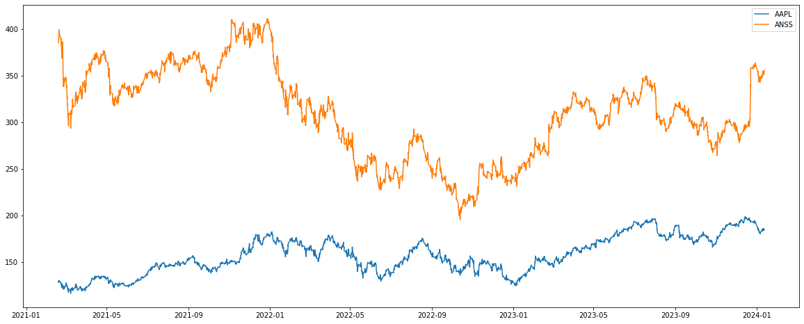
Adding % Change in Close Price columns
df1 = tech_companies[0][1]

df1['Close']
Datetime
2021-02-18 09:30:00-05:00 128.119904
2021-02-18 10:30:00-05:00 128.675705
2021-02-18 11:30:00-05:00 128.620102
2021-02-18 12:30:00-05:00 128.994995
2021-02-18 13:30:00-05:00 128.710007
...
2024-01-11 11:30:00-05:00 184.050003
2024-01-11 12:30:00-05:00 184.654999
2024-01-11 13:30:00-05:00 185.514999
2024-01-11 14:30:00-05:00 185.369995
2024-01-11 15:30:00-05:00 185.370102
Name: Close, Length: 5094, dtype: float64df1['Close'].shift(1)Datetime
2021-02-18 09:30:00-05:00 NaN
2021-02-18 10:30:00-05:00 128.119904
2021-02-18 11:30:00-05:00 128.675705
2021-02-18 12:30:00-05:00 128.620102
2021-02-18 13:30:00-05:00 128.994995
...
2024-01-11 11:30:00-05:00 184.190002
2024-01-11 12:30:00-05:00 184.050003
2024-01-11 13:30:00-05:00 184.654999
2024-01-11 14:30:00-05:00 185.514999
2024-01-11 15:30:00-05:00 185.369995
Name: Close, Length: 5094, dtype: float64temp_change_of_price = ((df1['Close'] - df1['Close'].shift(1)) / df1['Close'].shift(1))
temp_change_of_priceDatetime
2021-02-18 09:30:00-05:00 NaN
2021-02-18 10:30:00-05:00 4.338135e-03
2021-02-18 11:30:00-05:00 -4.321175e-04
2021-02-18 12:30:00-05:00 2.914732e-03
2021-02-18 13:30:00-05:00 -2.209298e-03
...
2024-01-11 11:30:00-05:00 -7.600814e-04
2024-01-11 12:30:00-05:00 3.287127e-03
2024-01-11 13:30:00-05:00 4.657337e-03
2024-01-11 14:30:00-05:00 -7.816310e-04
2024-01-11 15:30:00-05:00 5.762072e-07
Name: Close, Length: 5094, dtype: float64df1['% Change in Close Price'] = temp_change_of_price
df1['% Change in Close Price']Datetime
2021-02-18 09:30:00-05:00 NaN
2021-02-18 10:30:00-05:00 4.338135e-03
2021-02-18 11:30:00-05:00 -4.321175e-04
2021-02-18 12:30:00-05:00 2.914732e-03
2021-02-18 13:30:00-05:00 -2.209298e-03
...
2024-01-11 11:30:00-05:00 -7.600814e-04
2024-01-11 12:30:00-05:00 3.287127e-03
2024-01-11 13:30:00-05:00 4.657337e-03
2024-01-11 14:30:00-05:00 -7.816310e-04
2024-01-11 15:30:00-05:00 5.762072e-07
Name: % Change in Close Price, Length: 5094, dtype: float64# Initializing the dataframe of 2 stocks
df1 = tech_companies[0][1]
df2 = tech_companies[4][1]
# Create the % Change in Close price columns
df1['% Change in Close Price'] = None
df2['% Change in Close Price'] = None
# Using the change in price (current) and price (previous interval) and divided by the price (previous)
df1['% Change in Close Price'] = (df1['Close'] - df1['Close'].shift(1))/ df1['Close'].shift(1)
df2['% Change in Close Price'] = (df2['Close'] - df2['Close'].shift(1))/ df2['Close'].shift(1)
display(df1[['Close', '% Change in Close Price']])
display(df2[['Close', '% Change in Close Price']])# Removing top row as it is not needed and used.
df1 = df1[1:]
df2 = df2[1:]
display(df1[['Close', '% Change in Close Price']])
display(df2[['Close', '% Change in Close Price']])Plotting both the % Change in value of 2 stocks
plt.figure(figsize=(20, 8))
plt.plot(df1.index, df1['% Change in Close Price'],label=tech_companies[0][0])
plt.plot(df1.index, df2['% Change in Close Price'],label=tech_companies[4][0])
plt.legend()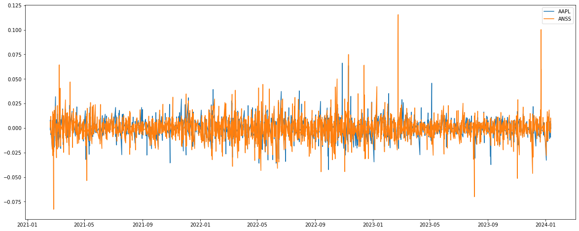
As compared to using only price, it can now be fairly compared. The spikes can be seen as large movement and these are the spikes that we would wish to identify. We can try to identify characteristics of such spikes, or even just above average returns. It also now resemble a lot like noise or random data with a very small hints of trends. Once the data is in this form, there are many ways we could further process this as well.
Frequency Distribution
When absolute price is plotted in a frequency distribution, it resemble a crown, because there are average prices that the stock will range between until some large price movement, shifting the average to another price level. Hence, it is like seeing multiple different normal distribution throughout.
plt.figure(figsize=(20, 7))

plt.hist(df1['Close'],bins=100,alpha=0.7,label=tech_companies[0][0])
plt.hist(df2['Close'],bins=100,alpha=0.7,label=tech_companies[4][0])
plt.legend()
plt.show()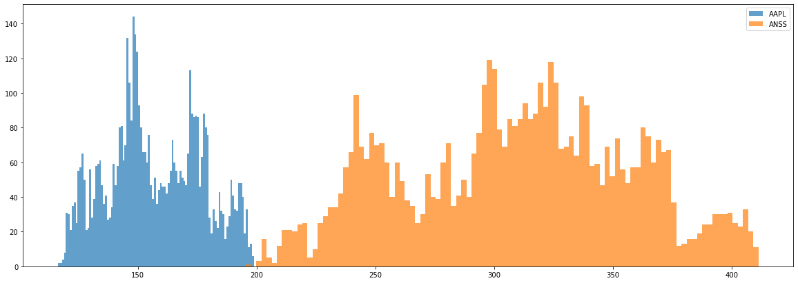
plt.figure(figsize=(20, 7))

plt.hist(df1['% Change in Close Price'],bins=100,label=tech_companies[0][0])
plt.hist(df2['% Change in Close Price'],bins=100,alpha=0.7,label=tech_companies[4][0])
plt.axvline(x = 0, linestyle = '-', color ='darkblue')
plt.legend()
plt.show()
plt.figure(figsize=(20, 7))

plt.hist(df1['% Change in Close Price'],bins=500,label=tech_companies[0][0])
plt.hist(df2['% Change in Close Price'],bins=500,alpha=0.7,label=tech_companies[4][0])
plt.axvline(x = 0, linestyle = '-', color ='darkblue')
plt.legend()
plt.show()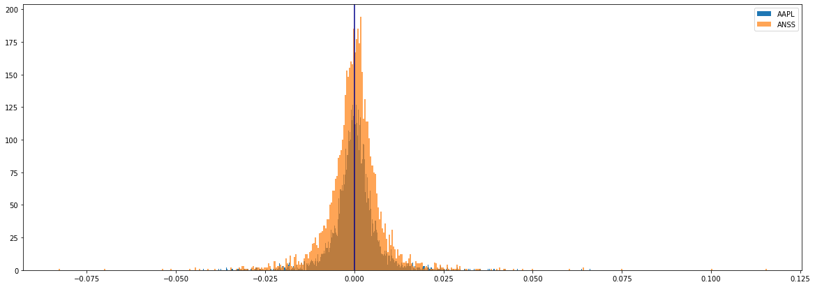
By using percentage change in price and plotting it in a frequency distribution, we can see that it resembles very much like a normal distribution. In a single glance we can see which stock has more price movement over the other. We can see if it is more skewed to downward price movements or positive movements. Exploration on using methods and models that can take advantage of the normal distribution would be advantageous but it will not be what we will do for this project.
Looking for patterns in % Change in Price, with % Change in Price
Next we will explore some patterns of the percentage change in price to see when it is going to have a positive or negative change. This is achieved by having a window size and desired return. The window size is how far back we want to look to identify a pattern and the desired return will be used as a threshold to filter on the minimum percentage change we would like to see. For example if we have a window size of three and desired return of five percent we will be looping through the percentage change. For each instance of five percent or more we will look back at the last 10 hours of percentage change.
Using the window size of 3 and desired return of 5%, we will use the example list below.
- It will loop through each value. The first value in the list that satisfies the desired return of five percent is the third element. Since we have a window size of three we cannot store the first instance. We continue looping until the next value which is the seventh element.
-
Store the last 3 values before 7%.
-
Then we continue the loop for the next value that satisfies the condition. The next one is the last value. We will then store the last three values.
- Which will give us the final list of
- Analyze the list. Given this toy example, we can see that a negative change, then a 2 percent change with a 3-4 percent change may lead to a high percent change.
We will explore using a 48 hour window with a desired return of three percent. This is a good number if we would like to have a higher chance of making a return. As shown in the frequency distribution above the higher the return the less likely it will occur. Furthermore if we were to use such a high return there will be too little data to create an average pattern.
# List to store the patterns found
patterns_of_higher_return = []
changes_in_price = df1['% Change in Close Price'].to_list()

# Setting window size and desired return
window_size = 48
desired_returns = 0.03

# Loop the column to find the those that have equal or more than desired returns
for row_no, returns in enumerate(changes_in_price):
    if row_no <= window_size:
        continue
    else:
        if returns >= desired_returns:
            patterns_of_higher_return.append(changes_in_price[row_no-window_size-1:row_no])

# List to store average pattern
average_pattern_of_higher_return = []

# Loop through a list from 0 to window size, indicating the value on the x axis
for no in range(window_size):
    temp = 0

    # Loop through the list of patterns and store all the value in the given x axis
    for pattern in patterns_of_higher_return:
        temp += pattern[no]

    # Get the average of the values collected in the given x axis
    average_pattern_of_higher_return.append(temp/len(patterns_of_higher_return))

# Set chart size
plt.figure(figsize=(15, 9))

# Plot the average
for i in patterns_of_higher_return:
    plt.plot(i,'C0',alpha=0.1)

# Plot the patterns found
plt.plot(average_pattern_of_higher_return,'darkblue',alpha=0.3,label='Average')
plt.scatter([x for x in range(window_size)],average_pattern_of_higher_return,color='darkblue',alpha=0.3,label='Average')
plt.xticks(np.arange(0, window_size, 2.0))
plt.legend()
plt.show()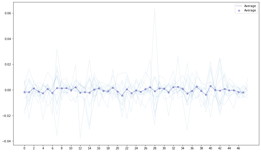
Using the same thing as above, but we look into patterns of losses, are there also patterns that can indicate a negative percentage change?
# List to store the patterns found
patterns_of_higher_losses = []
prices = df1['% Change in Close Price'].to_list()

# Setting window size and desired return
window_size = 48
desired_returns = -0.03

# Loop the column to find the those that have equal or more than desired returns
for row_no, returns in enumerate(prices):
    if row_no <= window_size:
        continue
    else:
        if returns <= desired_returns:
            patterns_of_higher_losses.append(prices[row_no-window_size-1:row_no])

# List to store average pattern
average_pattern_of_higher_losses = []

# Loop through a list from 0 to window size, indicating the value on the x axis
for no in range(window_size):
    temp = 0

    # Loop through the list of patterns and store all the value in the given x axis
    for pattern in patterns_of_higher_losses:
        temp += pattern[no]

    # Get the average of the values collected in the given x axis
    average_pattern_of_higher_losses.append(temp/len(patterns_of_higher_losses))

# Set chart size
plt.figure(figsize=(15,9))

# Plot the average
for i in patterns_of_higher_losses:
    plt.plot(i,'C0',alpha=0.1)

# Plot the patterns found
plt.plot(average_pattern_of_higher_losses,'darkblue',alpha=0.3,label='Average')
plt.scatter([x for x in range(window_size)],average_pattern_of_higher_losses,color='darkblue',alpha=0.3,label='Average')
plt.xticks(np.arange(0, window_size, 2.0))
plt.legend()
plt.show()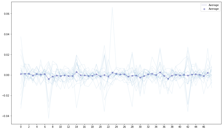
It seems like they do have different areas of peaks and trough. This means that these differences might be able to be used as early indicators for positive or negative change. We can have a clearer view by stacking both of them together.
# Set the chart size
plt.figure(figsize=(15,9))

# Plot both the averages
plt.plot(average_pattern_of_higher_losses)
plt.plot(average_pattern_of_higher_return)
plt.scatter([x for x in range(window_size)],average_pattern_of_higher_losses,color='darkblue',alpha=0.5,label='Average')
plt.scatter([x for x in range(window_size)],average_pattern_of_higher_return,color='darkorange',alpha=0.5,label='Average')
plt.xticks(np.arange(0, window_size, 2.0))
plt.show()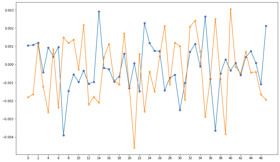
From here we might even be able to use some form of image recognition models or even use dynamic time warping to match the average recurring pattern found here to create a trading strategy. The difference between the pattern identifying a positive percentage change and a negative change seem to have some distinction. It can be seen that there are several areas of opposite values which can be used as an indicator that the next predicted value would be a positive or negative one.
Using Scaled Price
Using the same codes as above, we implement and explore what if we were to use price instead. We will need to scaled the pattern to values between 0 - 1, so that we can compare the different price movement occurring before the desired return. A 5% return but the pattern before it could [1,2,3] and [100,110,113]. If we do not scale the lists individually, we cannot see any meaningful difference among them.
patterns_of_higher_return = []
prices = df1['Close']
return_percentage = df1['% Change in Close Price'].to_list()

window_size = 48
desired_returns = 0.03

for row_no, returns in enumerate(return_percentage):
    if row_no <= window_size:
        continue
    else:
        if returns >= desired_returns:
            temp = prices[row_no-window_size:row_no]
            maxtemp = temp.max()
            mintemp = temp.min()

            patterns_of_higher_return.append(
                [((x-mintemp)/(maxtemp - mintemp))*1 for x in temp]
            )

average_pattern_of_higher_return = []

for no in range(window_size):
    temp = 0
    for pattern in patterns_of_higher_losses:
        temp += pattern[no]
    average_pattern_of_higher_losses.append(temp/len(patterns_of_higher_losses))

plt.figure(figsize=(20, 7))
x_values = [x for x in range(window_size)]

for i in patterns_of_higher_return:
    plt.plot(x_values,i,'C1',alpha=0.2)
plt.show()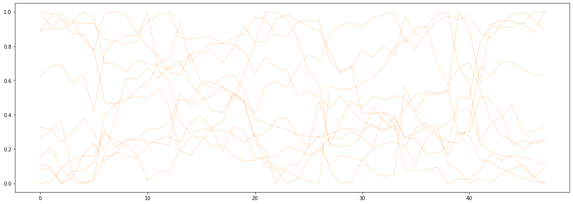
By using normal price, even when it is scaled, it is hard to further identify some form of repeatable pattern.
We will explore this again in the later part of the project, after extracting datetime features.
Adding % Change in Close Price for all stocks
change_in_close_price_str = '% Change in Close Price'
reference_column = 'Close'

print('Before adding the column:')
print('Number of Column: ', [len(tech_company[1].columns) for tech_company in tech_companies])

for tech_company in tech_companies:

    temp = tech_company[1]
    temp[change_in_close_price_str] = (temp[reference_column] - temp[reference_column].shift(1))/temp[reference_column].shift(1)
    tech_company[1][change_in_close_price_str] = temp[change_in_close_price_str]

print()

print('After adding the column:')
print('Number of Column: ', [len(tech_company[1].columns) for tech_company in tech_companies])
Before adding the column:
Number of Column: [8, 8, 8, 8, 8, 8, 8, 8, 8, 8, 8, 8, 8, 8, 8, 8, 8, 8, 8, 8, 8, 8, 8, 8, 8]
After adding the column:
Number of Column: [8, 8, 8, 8, 8, 8, 8, 8, 8, 8, 8, 8, 8, 8, 8, 8, 8, 8, 8, 8, 8, 8, 8, 8, 8]Processing all other price related columns
Open Price
change_in_close_price_str = '% Change in Open Price'
reference_column = 'Open'

print('Before adding the column:')
print('Number of Column: ', [len(tech_company[1].columns) for tech_company in tech_companies])

for tech_company in tech_companies:

    temp = tech_company[1]
    temp[change_in_close_price_str] = (temp[reference_column] - temp[reference_column].shift(1))/temp[reference_column].shift(1)
    tech_company[1][change_in_close_price_str] = temp[change_in_close_price_str]

print()

print('After adding the column:')
print('Number of Column: ', [len(tech_company[1].columns) for tech_company in tech_companies])
Before adding the column:
Number of Column: [8, 8, 8, 8, 8, 8, 8, 8, 8, 8, 8, 8, 8, 8, 8, 8, 8, 8, 8, 8, 8, 8, 8, 8, 8]
After adding the column:
Number of Column: [9, 9, 9, 9, 9, 9, 9, 9, 9, 9, 9, 9, 9, 9, 9, 9, 9, 9, 9, 9, 9, 9, 9, 9, 9]Low Price
change_in_close_price_str = '% Change in Low Price'
reference_column = 'Low'

print('Before adding the column:')
print('Number of Column: ', [len(tech_company[1].columns) for tech_company in tech_companies])

for tech_company in tech_companies:

    temp = tech_company[1]
    temp[change_in_close_price_str] = (temp[reference_column] - temp[reference_column].shift(1))/temp[reference_column].shift(1)
    tech_company[1][change_in_close_price_str] = temp[change_in_close_price_str]

print()

print('After adding the column:')
print('Number of Column: ', [len(tech_company[1].columns) for tech_company in tech_companies])
Before adding the column:
Number of Column: [9, 9, 9, 9, 9, 9, 9, 9, 9, 9, 9, 9, 9, 9, 9, 9, 9, 9, 9, 9, 9, 9, 9, 9, 9]
After adding the column:
Number of Column: [10, 10, 10, 10, 10, 10, 10, 10, 10, 10, 10, 10, 10, 10, 10, 10, 10, 10, 10, 10, 10, 10, 10, 10, 10]High Price
change_in_close_price_str = '% Change in High Price'
reference_column = 'High'

print('Before adding the column:')
print('Number of Column: ', [len(tech_company[1].columns) for tech_company in tech_companies])

for tech_company in tech_companies:

    temp = tech_company[1]
    temp[change_in_close_price_str] = (temp[reference_column] - temp[reference_column].shift(1))/temp[reference_column].shift(1)
    tech_company[1][change_in_close_price_str] = temp[change_in_close_price_str]

print()

print('After adding the column:')
print('Number of Column: ', [len(tech_company[1].columns) for tech_company in tech_companies])
Before adding the column:
Number of Column: [10, 10, 10, 10, 10, 10, 10, 10, 10, 10, 10, 10, 10, 10, 10, 10, 10, 10, 10, 10, 10, 10, 10, 10, 10]
After adding the column:
Number of Column: [11, 11, 11, 11, 11, 11, 11, 11, 11, 11, 11, 11, 11, 11, 11, 11, 11, 11, 11, 11, 11, 11, 11, 11, 11]tech_companies[0][1] Open High Low Close \
Datetime
2021-02-18 09:30:00-05:00 129.199997 129.679993 127.410004 128.119904
2021-02-18 10:30:00-05:00 128.100006 129.104996 127.830002 128.675705
2021-02-18 11:30:00-05:00 128.669998 128.710007 127.900002 128.620102
2021-02-18 12:30:00-05:00 128.625000 129.070007 128.449997 128.994995
2021-02-18 13:30:00-05:00 129.000000 129.050003 128.449997 128.710007
... ... ... ... ...
2024-01-11 11:30:00-05:00 184.184998 184.449997 183.835007 184.050003
2024-01-11 12:30:00-05:00 184.074997 184.777206 184.074997 184.654999
2024-01-11 13:30:00-05:00 184.669998 185.539993 184.559998 185.514999
2024-01-11 14:30:00-05:00 185.520004 185.699997 184.755005 185.369995
2024-01-11 15:30:00-05:00 185.369995 185.559998 185.350006 185.370102
Volume Dividends Stock Splits \
Datetime
2021-02-18 09:30:00-05:00 28938326 0.0 0.0
2021-02-18 10:30:00-05:00 13477687 0.0 0.0
2021-02-18 11:30:00-05:00 12770713 0.0 0.0
2021-02-18 12:30:00-05:00 8465690 0.0 0.0
2021-02-18 13:30:00-05:00 8516504 0.0 0.0
... ... ... ...
2024-01-11 11:30:00-05:00 3849444 0.0 0.0
2024-01-11 12:30:00-05:00 4000614 0.0 0.0
2024-01-11 13:30:00-05:00 3924789 0.0 0.0
2024-01-11 14:30:00-05:00 4502053 0.0 0.0
2024-01-11 15:30:00-05:00 1503923 0.0 0.0
% Change in Close Price % Change in Open Price \
Datetime
2021-02-18 09:30:00-05:00 NaN NaN
2021-02-18 10:30:00-05:00 4.338135e-03 -0.008514
2021-02-18 11:30:00-05:00 -4.321175e-04 0.004450
2021-02-18 12:30:00-05:00 2.914732e-03 -0.000350
2021-02-18 13:30:00-05:00 -2.209298e-03 0.002915
... ... ...
2024-01-11 11:30:00-05:00 -7.600814e-04 -0.000976
2024-01-11 12:30:00-05:00 3.287127e-03 -0.000597
2024-01-11 13:30:00-05:00 4.657337e-03 0.003232
2024-01-11 14:30:00-05:00 -7.816310e-04 0.004603
2024-01-11 15:30:00-05:00 5.762072e-07 -0.000809
% Change in Low Price % Change in High Price
Datetime
2021-02-18 09:30:00-05:00 NaN NaN
2021-02-18 10:30:00-05:00 0.003296 -0.004434
2021-02-18 11:30:00-05:00 0.000548 -0.003059
2021-02-18 12:30:00-05:00 0.004300 0.002797
2021-02-18 13:30:00-05:00 0.000000 -0.000155
... ... ...
2024-01-11 11:30:00-05:00 0.000000 -0.002326
2024-01-11 12:30:00-05:00 0.001305 0.001774
2024-01-11 13:30:00-05:00 0.002635 0.004128
2024-01-11 14:30:00-05:00 0.001057 0.000862
2024-01-11 15:30:00-05:00 0.003220 -0.000754
[5094 rows x 11 columns]Choosing Companies
Due to time and scope constraints we will be selecting the top three companies to further explore and perform implementation in the later parts of the coursework. The condition for picking out three companies is that these companies will need to provide the most opportunity to make a return. Therefore we look for companies not only with large price movements but also with high frequency of those movements. We need to establish that we will only be looking into buying shares or entering a long position. It is understood that money could also be made when the market moves downward. However the scope will be finding the highest absolute sum of percentage change in price as any direction is an opportunity to generate returns. We will limit our analysis to making returns when the market is going up.
Because our data is already processed to represent price movement there are several ways we can approach this.
- The sum of percentage change in price to see which company would have the highest net positive movement.
- The number of positive percentage changes in price to see which company would have the most frequent number of positive movements.
- The sum of positive percentage change in price to see which company would have the highest positive movement.
- The sum of the differences between high and low price.
- The sum of the differences between high and close price.
- The sum of the differences between low and close price.
We will be settling on using total positive percentage change.
We will also be comparing this to the approach of using standard deviation of the stock price. Standard deviation usually represents the volatility of a financial instrument and also risk. Therefore a stock with a higher standard deviation is what we would like to pick.
tech_companies[0][1]['% Change in Close Price']Datetime
2021-02-18 09:30:00-05:00 NaN
2021-02-18 10:30:00-05:00 4.338135e-03
2021-02-18 11:30:00-05:00 -4.321175e-04
2021-02-18 12:30:00-05:00 2.914732e-03
2021-02-18 13:30:00-05:00 -2.209298e-03
...
2024-01-11 11:30:00-05:00 -7.600814e-04
2024-01-11 12:30:00-05:00 3.287127e-03
2024-01-11 13:30:00-05:00 4.657337e-03
2024-01-11 14:30:00-05:00 -7.816310e-04
2024-01-11 15:30:00-05:00 5.762072e-07
Name: % Change in Close Price, Length: 5094, dtype: float64tech_companies_ticker = [tech_company[0] for tech_company in tech_companies]
companies_df = pd.DataFrame(index = tech_companies_ticker)
companies_dfEmpty DataFrame
Columns: []
Index: [AAPL, ADI, ADSK, AMD, ANSS, ASML, AVGO, CDW, CRWD, CTSH, DASH, DDOG, GOOG, GOOGL, KLAC, LRCX, MDB, META, MSFT, NVDA, NXPI, PANW, PDD, QCOM, TXN]Sum of % Positive Close Price Changes
sum_of_positive_changes_str = 'Sum of Positive Close Price Changes'
companies_df[sum_of_positive_changes_str] = None

for tech_company in tech_companies:
        companies_df.loc[tech_company[0], sum_of_positive_changes_str] = sum(
            list(filter(lambda x: x > 0, tech_company[1]['% Change in Close Price'][1:]))
        )

companies_df
Sum of Positive Close Price Changes
AAPL 10.784127
ADI 12.092185
ADSK 13.781926
AMD 19.563814
ANSS 12.933404
ASML 14.493156
AVGO 12.797733
CDW 10.444991
CRWD 20.581841
CTSH 9.911096
DASH 24.763219
DDOG 23.552644
GOOG 11.539979
GOOGL 11.683878
KLAC 15.823952
LRCX 16.54264
MDB 25.052964
META 15.01839
MSFT 10.795445
NVDA 20.052809
NXPI 15.32139
PANW 15.20349
PDD 24.920476
QCOM 13.922156
TXN 10.838171Sum of % Change in Price
sum_of_changes_str = 'Sum of Close Price Changes'
companies_df[sum_of_changes_str] = None

for tech_company in tech_companies:
        companies_df.loc[tech_company[0], sum_of_changes_str] = sum(tech_company[1]['% Change in Close Price'][1:])

companies_df
Sum of Positive Close Price Changes Sum of Close Price Changes
AAPL 10.784127 0.475806
ADI 12.092185 0.316209
ADSK 13.781926 0.002792
AMD 19.563814 0.867206
ANSS 12.933404 0.087076
ASML 14.493156 0.437682
AVGO 12.797733 0.975791
CDW 10.444991 0.43849
CRWD 20.581841 0.647721
CTSH 9.911096 0.105226
DASH 24.763219 0.055267
DDOG 23.552644 0.787556
GOOG 11.539979 0.442579
GOOGL 11.683878 0.439984
KLAC 15.823952 0.775045
LRCX 16.54264 0.544324
MDB 25.052964 0.714716
META 15.01839 0.625347
MSFT 10.795445 0.57566
NVDA 20.052809 1.695652
NXPI 15.32139 0.346168
PANW 15.20349 1.153684
PDD 24.920476 0.707896
QCOM 13.922156 0.1617
TXN 10.838171 0.051368Average Gap between Low and High
average_gap_str = 'Average Gap (High - Low)'
companies_df[average_gap_str] = None

for tech_company in tech_companies:
        companies_df.loc[tech_company[0], average_gap_str] = sum((tech_company[1]['High'][1:] - tech_company[1]['Low'][1:]) / tech_company[1]['Low'][1:] ) / len(tech_company[1][1:])

companies_df Sum of Positive Close Price Changes Sum of Close Price Changes \
AAPL 10.784127 0.475806
ADI 12.092185 0.316209
ADSK 13.781926 0.002792
AMD 19.563814 0.867206
ANSS 12.933404 0.087076
ASML 14.493156 0.437682
AVGO 12.797733 0.975791
CDW 10.444991 0.43849
CRWD 20.581841 0.647721
CTSH 9.911096 0.105226
DASH 24.763219 0.055267
DDOG 23.552644 0.787556
GOOG 11.539979 0.442579
GOOGL 11.683878 0.439984
KLAC 15.823952 0.775045
LRCX 16.54264 0.544324
MDB 25.052964 0.714716
META 15.01839 0.625347
MSFT 10.795445 0.57566
NVDA 20.052809 1.695652
NXPI 15.32139 0.346168
PANW 15.20349 1.153684
PDD 24.920476 0.707896
QCOM 13.922156 0.1617
TXN 10.838171 0.051368
Average Gap (High - Low)
AAPL 0.007524
ADI 0.008492
ADSK 0.009741
AMD 0.013881
ANSS 0.008775
ASML 0.008735
AVGO 0.008587
CDW 0.007192
CRWD 0.01487
CTSH 0.006904
DASH 0.018389
DDOG 0.016879
GOOG 0.007889
GOOGL 0.008093
KLAC 0.010719
LRCX 0.011346
MDB 0.017585
META 0.010453
MSFT 0.007331
NVDA 0.013883
NXPI 0.010598
PANW 0.010641
PDD 0.016798
QCOM 0.009806
TXN 0.007737Standard Deviation
columns = tech_companies[0][1].columns
index = [tech_company[0] for tech_company in tech_companies]
companies_standard_deviations = pd.DataFrame(columns=columns, index=index)

for tech_company in tech_companies:
    companies_standard_deviations.loc[tech_company[0]] = tech_company[1].std()

companies_standard_deviations = companies_standard_deviations.sort_values(['% Change in Close Price'], ascending=False).drop(columns=['Volume', 'Dividends', 'Stock Splits'])
companies_standard_deviations Open High Low Close % Change in Close Price \
PDD 32.080006 32.23114 31.915326 32.064646 0.019483
MDB 98.760671 99.268854 98.228868 98.727557 0.01708
DASH 50.425317 50.804168 50.037054 50.409624 0.01612
DDOG 30.319219 30.608159 30.01792 30.30877 0.015823
CRWD 47.528904 47.749702 47.289229 47.527375 0.013231
NVDA 114.239468 114.743463 113.70487 114.22924 0.012289
AMD 22.272153 22.431132 22.100393 22.267683 0.011628
META 80.131509 80.260925 79.970756 80.126257 0.01079
LRCX 96.648191 96.664046 96.555595 96.629964 0.010065
PANW 45.515648 45.717731 45.370409 45.561569 0.009816
KLAC 70.415159 70.490377 70.373619 70.452785 0.009329
ASML 101.669561 101.570227 101.722034 101.663423 0.009292
NXPI 21.07974 21.067232 21.073547 21.079791 0.009153
ADSK 42.976498 43.041587 42.898398 42.968848 0.008853
QCOM 19.359434 19.527088 19.197413 19.3657 0.008699
ANSS 48.050243 48.119773 47.967689 48.050613 0.008109
AVGO 165.6667 166.459976 165.076903 165.81627 0.007442
GOOGL 16.905788 16.896378 16.890284 16.892939 0.007365
GOOG 17.025381 17.013128 17.015443 17.014153 0.007266
ADI 13.984689 13.938348 14.03361 13.99286 0.007145
MSFT 39.978472 40.00587 39.961993 39.978433 0.006599
CTSH 8.970093 8.996426 8.937564 8.970886 0.006481
AAPL 19.769706 19.766775 19.782729 19.771827 0.006468
TXN 12.61352 12.58614 12.621553 12.616761 0.006416
CDW 16.664114 16.634817 16.694416 16.665404 0.006257
% Change in Open Price % Change in Low Price % Change in High Price
PDD 0.018998 0.019522 0.020066
MDB 0.017038 0.016511 0.017406
DASH 0.016489 0.016242 0.016296
DDOG 0.015958 0.015543 0.015966
CRWD 0.013339 0.013352 0.013045
NVDA 0.01249 0.011933 0.011902
AMD 0.011748 0.011282 0.01135
META 0.010954 0.010853 0.010767
LRCX 0.009959 0.009788 0.009623
PANW 0.009765 0.009607 0.009957
KLAC 0.009507 0.009162 0.009164
ASML 0.009398 0.009049 0.008881
NXPI 0.009172 0.008935 0.008639
ADSK 0.008846 0.00886 0.008613
QCOM 0.008886 0.008561 0.008529
ANSS 0.008587 0.008109 0.008235
AVGO 0.007365 0.007084 0.007253
GOOGL 0.007362 0.007163 0.007374
GOOG 0.007241 0.007052 0.006969
ADI 0.007332 0.007182 0.00674
MSFT 0.006522 0.006275 0.006274
CTSH 0.006628 0.00643 0.006285
AAPL 0.006413 0.006331 0.006053
TXN 0.006685 0.006363 0.005972
CDW 0.006454 0.006477 0.005878columns = companies_standard_deviations.columns[-4:]
companies_df[columns] = companies_standard_deviations[columns]
companies_df Sum of Positive Close Price Changes Sum of Close Price Changes \
AAPL 10.784127 0.475806
ADI 12.092185 0.316209
ADSK 13.781926 0.002792
AMD 19.563814 0.867206
ANSS 12.933404 0.087076
ASML 14.493156 0.437682
AVGO 12.797733 0.975791
CDW 10.444991 0.43849
CRWD 20.581841 0.647721
CTSH 9.911096 0.105226
DASH 24.763219 0.055267
DDOG 23.552644 0.787556
GOOG 11.539979 0.442579
GOOGL 11.683878 0.439984
KLAC 15.823952 0.775045
LRCX 16.54264 0.544324
MDB 25.052964 0.714716
META 15.01839 0.625347
MSFT 10.795445 0.57566
NVDA 20.052809 1.695652
NXPI 15.32139 0.346168
PANW 15.20349 1.153684
PDD 24.920476 0.707896
QCOM 13.922156 0.1617
TXN 10.838171 0.051368
Average Gap (High - Low) % Change in Close Price % Change in Open Price \
AAPL 0.007524 0.006468 0.006413
ADI 0.008492 0.007145 0.007332
ADSK 0.009741 0.008853 0.008846
AMD 0.013881 0.011628 0.011748
ANSS 0.008775 0.008109 0.008587
ASML 0.008735 0.009292 0.009398
AVGO 0.008587 0.007442 0.007365
CDW 0.007192 0.006257 0.006454
CRWD 0.01487 0.013231 0.013339
CTSH 0.006904 0.006481 0.006628
DASH 0.018389 0.01612 0.016489
DDOG 0.016879 0.015823 0.015958
GOOG 0.007889 0.007266 0.007241
GOOGL 0.008093 0.007365 0.007362
KLAC 0.010719 0.009329 0.009507
LRCX 0.011346 0.010065 0.009959
MDB 0.017585 0.01708 0.017038
META 0.010453 0.01079 0.010954
MSFT 0.007331 0.006599 0.006522
NVDA 0.013883 0.012289 0.01249
NXPI 0.010598 0.009153 0.009172
PANW 0.010641 0.009816 0.009765
PDD 0.016798 0.019483 0.018998
QCOM 0.009806 0.008699 0.008886
TXN 0.007737 0.006416 0.006685
% Change in Low Price % Change in High Price
AAPL 0.006331 0.006053
ADI 0.007182 0.00674
ADSK 0.00886 0.008613
AMD 0.011282 0.01135
ANSS 0.008109 0.008235
ASML 0.009049 0.008881
AVGO 0.007084 0.007253
CDW 0.006477 0.005878
CRWD 0.013352 0.013045
CTSH 0.00643 0.006285
DASH 0.016242 0.016296
DDOG 0.015543 0.015966
GOOG 0.007052 0.006969
GOOGL 0.007163 0.007374
KLAC 0.009162 0.009164
LRCX 0.009788 0.009623
MDB 0.016511 0.017406
META 0.010853 0.010767
MSFT 0.006275 0.006274
NVDA 0.011933 0.011902
NXPI 0.008935 0.008639
PANW 0.009607 0.009957
PDD 0.019522 0.020066
QCOM 0.008561 0.008529
TXN 0.006363 0.005972Any of the columns available in the DataFrame are all justifiable to be used to decide. But we will go through each of them to see which are the companies that have more price movement that others.
Comparing the columns
We will create a column to see how many points can the companies collect. The top 3 highest scorer will be chosen to be used, moving forward
companies_df['Score'] = 0
companies_df Sum of Positive Close Price Changes Sum of Close Price Changes \
AAPL 10.784127 0.475806
ADI 12.092185 0.316209
ADSK 13.781926 0.002792
AMD 19.563814 0.867206
ANSS 12.933404 0.087076
ASML 14.493156 0.437682
AVGO 12.797733 0.975791
CDW 10.444991 0.43849
CRWD 20.581841 0.647721
CTSH 9.911096 0.105226
DASH 24.763219 0.055267
DDOG 23.552644 0.787556
GOOG 11.539979 0.442579
GOOGL 11.683878 0.439984
KLAC 15.823952 0.775045
LRCX 16.54264 0.544324
MDB 25.052964 0.714716
META 15.01839 0.625347
MSFT 10.795445 0.57566
NVDA 20.052809 1.695652
NXPI 15.32139 0.346168
PANW 15.20349 1.153684
PDD 24.920476 0.707896
QCOM 13.922156 0.1617
TXN 10.838171 0.051368
Average Gap (High - Low) % Change in Close Price % Change in Open Price \
AAPL 0.007524 0.006468 0.006413
ADI 0.008492 0.007145 0.007332
ADSK 0.009741 0.008853 0.008846
AMD 0.013881 0.011628 0.011748
ANSS 0.008775 0.008109 0.008587
ASML 0.008735 0.009292 0.009398
AVGO 0.008587 0.007442 0.007365
CDW 0.007192 0.006257 0.006454
CRWD 0.01487 0.013231 0.013339
CTSH 0.006904 0.006481 0.006628
DASH 0.018389 0.01612 0.016489
DDOG 0.016879 0.015823 0.015958
GOOG 0.007889 0.007266 0.007241
GOOGL 0.008093 0.007365 0.007362
KLAC 0.010719 0.009329 0.009507
LRCX 0.011346 0.010065 0.009959
MDB 0.017585 0.01708 0.017038
META 0.010453 0.01079 0.010954
MSFT 0.007331 0.006599 0.006522
NVDA 0.013883 0.012289 0.01249
NXPI 0.010598 0.009153 0.009172
PANW 0.010641 0.009816 0.009765
PDD 0.016798 0.019483 0.018998
QCOM 0.009806 0.008699 0.008886
TXN 0.007737 0.006416 0.006685
% Change in Low Price % Change in High Price Score
AAPL 0.006331 0.006053 0
ADI 0.007182 0.00674 0
ADSK 0.00886 0.008613 0
AMD 0.011282 0.01135 0
ANSS 0.008109 0.008235 0
ASML 0.009049 0.008881 0
AVGO 0.007084 0.007253 0
CDW 0.006477 0.005878 0
CRWD 0.013352 0.013045 0
CTSH 0.00643 0.006285 0
DASH 0.016242 0.016296 0
DDOG 0.015543 0.015966 0
GOOG 0.007052 0.006969 0
GOOGL 0.007163 0.007374 0
KLAC 0.009162 0.009164 0
LRCX 0.009788 0.009623 0
MDB 0.016511 0.017406 0
META 0.010853 0.010767 0
MSFT 0.006275 0.006274 0
NVDA 0.011933 0.011902 0
NXPI 0.008935 0.008639 0
PANW 0.009607 0.009957 0
PDD 0.019522 0.020066 0
QCOM 0.008561 0.008529 0
TXN 0.006363 0.005972 0companies_df.columns[-1]'Score'# Looping through all the columns in the DataFrame
for column in companies_df.columns:
# Sorting them in descending order
companies_df = companies_df.sort_values(column,ascending=False)
# Giving a point to the top 3 companies
companies_df.iloc[:3, -1] += 1
companies_df Sum of Positive Close Price Changes Sum of Close Price Changes \
DASH 24.763219 0.055267
MDB 25.052964 0.714716
PDD 24.920476 0.707896
DDOG 23.552644 0.787556
NVDA 20.052809 1.695652
PANW 15.20349 1.153684
AVGO 12.797733 0.975791
ANSS 12.933404 0.087076
TXN 10.838171 0.051368
AAPL 10.784127 0.475806
MSFT 10.795445 0.57566
CTSH 9.911096 0.105226
ADI 12.092185 0.316209
GOOG 11.539979 0.442579
GOOGL 11.683878 0.439984
NXPI 15.32139 0.346168
QCOM 13.922156 0.1617
ADSK 13.781926 0.002792
ASML 14.493156 0.437682
KLAC 15.823952 0.775045
LRCX 16.54264 0.544324
META 15.01839 0.625347
AMD 19.563814 0.867206
CRWD 20.581841 0.647721
CDW 10.444991 0.43849
Average Gap (High - Low) % Change in Close Price % Change in Open Price \
DASH 0.018389 0.01612 0.016489
MDB 0.017585 0.01708 0.017038
PDD 0.016798 0.019483 0.018998
DDOG 0.016879 0.015823 0.015958
NVDA 0.013883 0.012289 0.01249
PANW 0.010641 0.009816 0.009765
AVGO 0.008587 0.007442 0.007365
ANSS 0.008775 0.008109 0.008587
TXN 0.007737 0.006416 0.006685
AAPL 0.007524 0.006468 0.006413
MSFT 0.007331 0.006599 0.006522
CTSH 0.006904 0.006481 0.006628
ADI 0.008492 0.007145 0.007332
GOOG 0.007889 0.007266 0.007241
GOOGL 0.008093 0.007365 0.007362
NXPI 0.010598 0.009153 0.009172
QCOM 0.009806 0.008699 0.008886
ADSK 0.009741 0.008853 0.008846
ASML 0.008735 0.009292 0.009398
KLAC 0.010719 0.009329 0.009507
LRCX 0.011346 0.010065 0.009959
META 0.010453 0.01079 0.010954
AMD 0.013881 0.011628 0.011748
CRWD 0.01487 0.013231 0.013339
CDW 0.007192 0.006257 0.006454
% Change in Low Price % Change in High Price Score
DASH 0.016242 0.016296 7
MDB 0.016511 0.017406 7
PDD 0.019522 0.020066 6
DDOG 0.015543 0.015966 1
NVDA 0.011933 0.011902 1
PANW 0.009607 0.009957 1
AVGO 0.007084 0.007253 1
ANSS 0.008109 0.008235 0
TXN 0.006363 0.005972 0
AAPL 0.006331 0.006053 0
MSFT 0.006275 0.006274 0
CTSH 0.00643 0.006285 0
ADI 0.007182 0.00674 0
GOOG 0.007052 0.006969 0
GOOGL 0.007163 0.007374 0
NXPI 0.008935 0.008639 0
QCOM 0.008561 0.008529 0
ADSK 0.00886 0.008613 0
ASML 0.009049 0.008881 0
KLAC 0.009162 0.009164 0
LRCX 0.009788 0.009623 0
META 0.010853 0.010767 0
AMD 0.011282 0.01135 0
CRWD 0.013352 0.013045 0
CDW 0.006477 0.005878 0Based on the results, we can see that ticker 'MDB', 'PDD' and 'DASH' are the winners as they scored the most.
winning_companies = ['MDB', 'PDD', 'DASH']
companies_dict = {}

for tech_company in tech_companies:
    if tech_company[0] in winning_companies:
        companies_dict[tech_company[0]] = tech_company[1]

companies_dict{'DASH': Open High Low Close \
Datetime
2021-02-18 09:30:00-05:00 194.300003 196.610001 188.990005 189.800003
2021-02-18 10:30:00-05:00 189.576096 194.800003 188.910004 193.691101
2021-02-18 11:30:00-05:00 193.770004 196.979996 191.339996 191.554993
2021-02-18 12:30:00-05:00 191.339996 194.490005 191.169998 193.899994
2021-02-18 13:30:00-05:00 194.149994 196.440002 193.809998 196.220001
... ... ... ... ...
2024-01-11 11:30:00-05:00 102.565002 103.139999 102.400002 102.925003
2024-01-11 12:30:00-05:00 102.959999 103.959999 102.889999 103.800003
2024-01-11 13:30:00-05:00 103.779999 104.650002 103.675003 104.625000
2024-01-11 14:30:00-05:00 104.644997 104.695000 104.065002 104.339996
2024-01-11 15:30:00-05:00 104.320000 104.330002 104.029999 104.100098
Volume Dividends Stock Splits \
Datetime
2021-02-18 09:30:00-05:00 410371 0.0 0.0
2021-02-18 10:30:00-05:00 270042 0.0 0.0
2021-02-18 11:30:00-05:00 270798 0.0 0.0
2021-02-18 12:30:00-05:00 185655 0.0 0.0
2021-02-18 13:30:00-05:00 108898 0.0 0.0
... ... ... ...
2024-01-11 11:30:00-05:00 226748 0.0 0.0
2024-01-11 12:30:00-05:00 230721 0.0 0.0
2024-01-11 13:30:00-05:00 270964 0.0 0.0
2024-01-11 14:30:00-05:00 247590 0.0 0.0
2024-01-11 15:30:00-05:00 87951 0.0 0.0
% Change in Close Price % Change in Open Price \
Datetime
2021-02-18 09:30:00-05:00 NaN NaN
2021-02-18 10:30:00-05:00 0.020501 -0.024312
2021-02-18 11:30:00-05:00 -0.011028 0.022123
2021-02-18 12:30:00-05:00 0.012242 -0.012541
2021-02-18 13:30:00-05:00 0.011965 0.014686
... ... ...
2024-01-11 11:30:00-05:00 0.003559 -0.012088
2024-01-11 12:30:00-05:00 0.008501 0.003851
2024-01-11 13:30:00-05:00 0.007948 0.007964
2024-01-11 14:30:00-05:00 -0.002724 0.008335
2024-01-11 15:30:00-05:00 -0.002299 -0.003106
% Change in Low Price % Change in High Price
Datetime
2021-02-18 09:30:00-05:00 NaN NaN
2021-02-18 10:30:00-05:00 -0.000423 -0.009206
2021-02-18 11:30:00-05:00 0.012863 0.011191
2021-02-18 12:30:00-05:00 -0.000888 -0.012641
2021-02-18 13:30:00-05:00 0.013810 0.010026
... ... ...
2024-01-11 11:30:00-05:00 -0.001073 -0.011596
2024-01-11 12:30:00-05:00 0.004785 0.007950
2024-01-11 13:30:00-05:00 0.007630 0.006637
2024-01-11 14:30:00-05:00 0.003762 0.000430
2024-01-11 15:30:00-05:00 -0.000336 -0.003486
[5094 rows x 11 columns],
'MDB': Open High Low Close \
Datetime
2021-02-18 09:30:00-05:00 402.079987 409.820007 397.397491 398.625000
2021-02-18 10:30:00-05:00 399.190002 407.035004 397.420013 404.570007
2021-02-18 11:30:00-05:00 405.480011 405.480011 401.940002 403.084991
2021-02-18 12:30:00-05:00 403.019989 404.109985 398.540009 403.070007
2021-02-18 13:30:00-05:00 402.799988 403.959991 402.029999 402.489990
... ... ... ... ...
2024-01-11 11:30:00-05:00 385.250000 387.010010 383.200012 383.899994
2024-01-11 12:30:00-05:00 384.160004 390.000000 384.010010 389.619995
2024-01-11 13:30:00-05:00 389.559998 393.489990 389.006989 392.549988
2024-01-11 14:30:00-05:00 392.679993 393.129913 391.830109 392.720001
2024-01-11 15:30:00-05:00 392.829987 393.519989 392.470001 393.494995
Volume Dividends Stock Splits \
Datetime
2021-02-18 09:30:00-05:00 108932 0.0 0.0
2021-02-18 10:30:00-05:00 59993 0.0 0.0
2021-02-18 11:30:00-05:00 41952 0.0 0.0
2021-02-18 12:30:00-05:00 79363 0.0 0.0
2021-02-18 13:30:00-05:00 59128 0.0 0.0
... ... ... ...
2024-01-11 11:30:00-05:00 133670 0.0 0.0
2024-01-11 12:30:00-05:00 90468 0.0 0.0
2024-01-11 13:30:00-05:00 112940 0.0 0.0
2024-01-11 14:30:00-05:00 102012 0.0 0.0
2024-01-11 15:30:00-05:00 45298 0.0 0.0
% Change in Close Price % Change in Open Price \
Datetime
2021-02-18 09:30:00-05:00 NaN NaN
2021-02-18 10:30:00-05:00 0.014914 -0.007188
2021-02-18 11:30:00-05:00 -0.003671 0.015757
2021-02-18 12:30:00-05:00 -0.000037 -0.006067
2021-02-18 13:30:00-05:00 -0.001439 -0.000546
... ... ...
2024-01-11 11:30:00-05:00 -0.003375 -0.009691
2024-01-11 12:30:00-05:00 0.014900 -0.002829
2024-01-11 13:30:00-05:00 0.007520 0.014057
2024-01-11 14:30:00-05:00 0.000433 0.008009
2024-01-11 15:30:00-05:00 0.001973 0.000382
% Change in Low Price % Change in High Price
Datetime
2021-02-18 09:30:00-05:00 NaN NaN
2021-02-18 10:30:00-05:00 0.000057 -0.006796
2021-02-18 11:30:00-05:00 0.011373 -0.003820
2021-02-18 12:30:00-05:00 -0.008459 -0.003379
2021-02-18 13:30:00-05:00 0.008757 -0.000371
... ... ...
2024-01-11 11:30:00-05:00 -0.005192 -0.009457
2024-01-11 12:30:00-05:00 0.002114 0.007726
2024-01-11 13:30:00-05:00 0.013013 0.008949
2024-01-11 14:30:00-05:00 0.007257 -0.000915
2024-01-11 15:30:00-05:00 0.001633 0.000992
[5094 rows x 11 columns],
'PDD': Open High Low Close \
Datetime
2021-02-18 09:30:00-05:00 198.000000 199.309998 192.899994 194.009995
2021-02-18 10:30:00-05:00 194.000000 196.000000 193.875000 195.100006
2021-02-18 11:30:00-05:00 195.000000 195.578003 193.100006 193.845001
2021-02-18 12:30:00-05:00 193.820007 195.544998 192.029999 195.220001
2021-02-18 13:30:00-05:00 195.179993 195.699997 194.660004 195.070007
... ... ... ... ...
2024-01-11 11:30:00-05:00 150.289993 151.050003 149.949997 150.550003
2024-01-11 12:30:00-05:00 150.554993 151.339996 150.475006 151.070007
2024-01-11 13:30:00-05:00 151.085007 151.630005 151.050003 151.539993
2024-01-11 14:30:00-05:00 151.559998 151.774994 151.430099 151.580994
2024-01-11 15:30:00-05:00 151.589996 151.720001 151.483994 151.649994
Volume Dividends Stock Splits \
Datetime
2021-02-18 09:30:00-05:00 1851955 0.0 0.0
2021-02-18 10:30:00-05:00 633548 0.0 0.0
2021-02-18 11:30:00-05:00 305243 0.0 0.0
2021-02-18 12:30:00-05:00 521230 0.0 0.0
2021-02-18 13:30:00-05:00 185892 0.0 0.0
... ... ... ...
2024-01-11 11:30:00-05:00 437558 0.0 0.0
2024-01-11 12:30:00-05:00 321022 0.0 0.0
2024-01-11 13:30:00-05:00 361665 0.0 0.0
2024-01-11 14:30:00-05:00 449250 0.0 0.0
2024-01-11 15:30:00-05:00 155503 0.0 0.0
% Change in Close Price % Change in Open Price \
Datetime
2021-02-18 09:30:00-05:00 NaN NaN
2021-02-18 10:30:00-05:00 0.005618 -0.020202
2021-02-18 11:30:00-05:00 -0.006433 0.005155
2021-02-18 12:30:00-05:00 0.007093 -0.006051
2021-02-18 13:30:00-05:00 -0.000768 0.007017
... ... ...
2024-01-11 11:30:00-05:00 0.001830 -0.006249
2024-01-11 12:30:00-05:00 0.003454 0.001763
2024-01-11 13:30:00-05:00 0.003111 0.003520
2024-01-11 14:30:00-05:00 0.000271 0.003144
2024-01-11 15:30:00-05:00 0.000455 0.000198
% Change in Low Price % Change in High Price
Datetime
2021-02-18 09:30:00-05:00 NaN NaN
2021-02-18 10:30:00-05:00 0.005054 -0.016607
2021-02-18 11:30:00-05:00 -0.003997 -0.002153
2021-02-18 12:30:00-05:00 -0.005541 -0.000169
2021-02-18 13:30:00-05:00 0.013696 0.000793
... ... ...
2024-01-11 11:30:00-05:00 0.000801 -0.003529
2024-01-11 12:30:00-05:00 0.003501 0.001920
2024-01-11 13:30:00-05:00 0.003821 0.001916
2024-01-11 14:30:00-05:00 0.002516 0.000956
2024-01-11 15:30:00-05:00 0.000356 -0.000362
[5094 rows x 11 columns]}Including Gap
As done above, we explored that the average gap between the high and low prices can also be an indication of price movement. Because our final dataset will be using change in price, the information about the difference between the high price and low price will be lost. Therefore, we should add a column that mentions the gap. Similarly, because the gap is based on the price, it shares the same issue as every price related column. But percentage change of the gap also does not convey the gap in price. Therefore, we will be using gap (difference between high and low) divided by the low price. Therefore, the gap is shown in percentage form.
companies_dict['MDB'].columnsIndex(['Open', 'High', 'Low', 'Close', 'Volume', 'Dividends', 'Stock Splits',
'% Change in Close Price', '% Change in Open Price',
'% Change in Low Price', '% Change in High Price'],
dtype='object')for company in winning_companies:
companies_dict[company]['Gap'] = (companies_dict[company]['High'] - companies_dict[company]['Low']) / companies_dict[company]['Low']
print(companies_dict[company]['Gap'])Datetime
2021-02-18 09:30:00-05:00 0.031260
2021-02-18 10:30:00-05:00 0.024194
2021-02-18 11:30:00-05:00 0.008807
2021-02-18 12:30:00-05:00 0.013976
2021-02-18 13:30:00-05:00 0.004801
...
2024-01-11 11:30:00-05:00 0.009943
2024-01-11 12:30:00-05:00 0.015599
2024-01-11 13:30:00-05:00 0.011524
2024-01-11 14:30:00-05:00 0.003317
2024-01-11 15:30:00-05:00 0.002675
Name: Gap, Length: 5094, dtype: float64
Datetime
2021-02-18 09:30:00-05:00 0.033230
2021-02-18 10:30:00-05:00 0.010961
2021-02-18 11:30:00-05:00 0.012833
2021-02-18 12:30:00-05:00 0.018304
2021-02-18 13:30:00-05:00 0.005343
...
2024-01-11 11:30:00-05:00 0.007336
2024-01-11 12:30:00-05:00 0.005748
2024-01-11 13:30:00-05:00 0.003840
2024-01-11 14:30:00-05:00 0.002278
2024-01-11 15:30:00-05:00 0.001558
Name: Gap, Length: 5094, dtype: float64
Datetime
2021-02-18 09:30:00-05:00 0.040320
2021-02-18 10:30:00-05:00 0.031179
2021-02-18 11:30:00-05:00 0.029476
2021-02-18 12:30:00-05:00 0.017367
2021-02-18 13:30:00-05:00 0.013570
...
2024-01-11 11:30:00-05:00 0.007227
2024-01-11 12:30:00-05:00 0.010399
2024-01-11 13:30:00-05:00 0.009404
2024-01-11 14:30:00-05:00 0.006054
2024-01-11 15:30:00-05:00 0.002884
Name: Gap, Length: 5094, dtype: float64Datetime Features
We will now be extracting the datetime features. This is because they might be repeating patterns within the datetime that are might not be obvious to us. For example, it may be most volatile during Tuesday, 2pm to 4pm, when there change in close of at least 3%. Therefore, extracting these features will allow the machine learning model to identify patterns as mentioned.
companies_dict['DASH'] Open High Low Close \
Datetime
2021-02-18 09:30:00-05:00 194.300003 196.610001 188.990005 189.800003
2021-02-18 10:30:00-05:00 189.576096 194.800003 188.910004 193.691101
2021-02-18 11:30:00-05:00 193.770004 196.979996 191.339996 191.554993
2021-02-18 12:30:00-05:00 191.339996 194.490005 191.169998 193.899994
2021-02-18 13:30:00-05:00 194.149994 196.440002 193.809998 196.220001
... ... ... ... ...
2024-01-11 11:30:00-05:00 102.565002 103.139999 102.400002 102.925003
2024-01-11 12:30:00-05:00 102.959999 103.959999 102.889999 103.800003
2024-01-11 13:30:00-05:00 103.779999 104.650002 103.675003 104.625000
2024-01-11 14:30:00-05:00 104.644997 104.695000 104.065002 104.339996
2024-01-11 15:30:00-05:00 104.320000 104.330002 104.029999 104.100098
Volume Dividends Stock Splits \
Datetime
2021-02-18 09:30:00-05:00 410371 0.0 0.0
2021-02-18 10:30:00-05:00 270042 0.0 0.0
2021-02-18 11:30:00-05:00 270798 0.0 0.0
2021-02-18 12:30:00-05:00 185655 0.0 0.0
2021-02-18 13:30:00-05:00 108898 0.0 0.0
... ... ... ...
2024-01-11 11:30:00-05:00 226748 0.0 0.0
2024-01-11 12:30:00-05:00 230721 0.0 0.0
2024-01-11 13:30:00-05:00 270964 0.0 0.0
2024-01-11 14:30:00-05:00 247590 0.0 0.0
2024-01-11 15:30:00-05:00 87951 0.0 0.0
% Change in Close Price % Change in Open Price \
Datetime
2021-02-18 09:30:00-05:00 NaN NaN
2021-02-18 10:30:00-05:00 0.020501 -0.024312
2021-02-18 11:30:00-05:00 -0.011028 0.022123
2021-02-18 12:30:00-05:00 0.012242 -0.012541
2021-02-18 13:30:00-05:00 0.011965 0.014686
... ... ...
2024-01-11 11:30:00-05:00 0.003559 -0.012088
2024-01-11 12:30:00-05:00 0.008501 0.003851
2024-01-11 13:30:00-05:00 0.007948 0.007964
2024-01-11 14:30:00-05:00 -0.002724 0.008335
2024-01-11 15:30:00-05:00 -0.002299 -0.003106
% Change in Low Price % Change in High Price \
Datetime
2021-02-18 09:30:00-05:00 NaN NaN
2021-02-18 10:30:00-05:00 -0.000423 -0.009206
2021-02-18 11:30:00-05:00 0.012863 0.011191
2021-02-18 12:30:00-05:00 -0.000888 -0.012641
2021-02-18 13:30:00-05:00 0.013810 0.010026
... ... ...
2024-01-11 11:30:00-05:00 -0.001073 -0.011596
2024-01-11 12:30:00-05:00 0.004785 0.007950
2024-01-11 13:30:00-05:00 0.007630 0.006637
2024-01-11 14:30:00-05:00 0.003762 0.000430
2024-01-11 15:30:00-05:00 -0.000336 -0.003486
Gap
Datetime
2021-02-18 09:30:00-05:00 0.040320
2021-02-18 10:30:00-05:00 0.031179
2021-02-18 11:30:00-05:00 0.029476
2021-02-18 12:30:00-05:00 0.017367
2021-02-18 13:30:00-05:00 0.013570
... ...
2024-01-11 11:30:00-05:00 0.007227
2024-01-11 12:30:00-05:00 0.010399
2024-01-11 13:30:00-05:00 0.009404
2024-01-11 14:30:00-05:00 0.006054
2024-01-11 15:30:00-05:00 0.002884
[5094 rows x 12 columns]for company in winning_companies:
# Add the DataTime information from index
companies_dict[company]['DateTime'] = companies_dict[company].index
# Extracting the Date Time Features
companies_dict[company]['Hour'] = companies_dict[company]['DateTime'].dt.hour
companies_dict[company]['Day'] = companies_dict[company]['DateTime'].dt.day
companies_dict[company]['Day_of_Week'] = companies_dict[company]['DateTime'].dt.day_of_week
companies_dict[company]['Month'] = companies_dict[company]['DateTime'].dt.month
companies_dict[company]['Quarter'] = companies_dict[company]['DateTime'].dt.quarter
# Drop the 'DateTime' column that was created
companies_dict[company] = companies_dict[company].drop('DateTime', axis = 1)
# Drop the top row - because when changing to percentage change in price, the top row has null values
companies_dict[company] = companies_dict[company][1:]
# Drop the columns that are not used
companies_dict[company] = companies_dict[company][companies_dict[company].columns[7:]]companies_dict['MDB'] % Change in Close Price % Change in Open Price \
Datetime
2021-02-18 10:30:00-05:00 0.014914 -0.007188
2021-02-18 11:30:00-05:00 -0.003671 0.015757
2021-02-18 12:30:00-05:00 -0.000037 -0.006067
2021-02-18 13:30:00-05:00 -0.001439 -0.000546
2021-02-18 14:30:00-05:00 -0.000447 -0.001912
... ... ...
2024-01-11 11:30:00-05:00 -0.003375 -0.009691
2024-01-11 12:30:00-05:00 0.014900 -0.002829
2024-01-11 13:30:00-05:00 0.007520 0.014057
2024-01-11 14:30:00-05:00 0.000433 0.008009
2024-01-11 15:30:00-05:00 0.001973 0.000382
% Change in Low Price % Change in High Price \
Datetime
2021-02-18 10:30:00-05:00 0.000057 -0.006796
2021-02-18 11:30:00-05:00 0.011373 -0.003820
2021-02-18 12:30:00-05:00 -0.008459 -0.003379
2021-02-18 13:30:00-05:00 0.008757 -0.000371
2021-02-18 14:30:00-05:00 -0.002375 -0.001634
... ... ...
2024-01-11 11:30:00-05:00 -0.005192 -0.009457
2024-01-11 12:30:00-05:00 0.002114 0.007726
2024-01-11 13:30:00-05:00 0.013013 0.008949
2024-01-11 14:30:00-05:00 0.007257 -0.000915
2024-01-11 15:30:00-05:00 0.001633 0.000992
Gap Hour Day Day_of_Week Month Quarter
Datetime
2021-02-18 10:30:00-05:00 0.024194 10 18 3 2 1
2021-02-18 11:30:00-05:00 0.008807 11 18 3 2 1
2021-02-18 12:30:00-05:00 0.013976 12 18 3 2 1
2021-02-18 13:30:00-05:00 0.004801 13 18 3 2 1
2021-02-18 14:30:00-05:00 0.005548 14 18 3 2 1
... ... ... ... ... ... ...
2024-01-11 11:30:00-05:00 0.009943 11 11 3 1 1
2024-01-11 12:30:00-05:00 0.015599 12 11 3 1 1
2024-01-11 13:30:00-05:00 0.011524 13 11 3 1 1
2024-01-11 14:30:00-05:00 0.003317 14 11 3 1 1
2024-01-11 15:30:00-05:00 0.002675 15 11 3 1 1
[5093 rows x 10 columns]companies_dict['PDD'] % Change in Close Price % Change in Open Price \
Datetime
2021-02-18 10:30:00-05:00 0.005618 -0.020202
2021-02-18 11:30:00-05:00 -0.006433 0.005155
2021-02-18 12:30:00-05:00 0.007093 -0.006051
2021-02-18 13:30:00-05:00 -0.000768 0.007017
2021-02-18 14:30:00-05:00 0.003025 -0.000461
... ... ...
2024-01-11 11:30:00-05:00 0.001830 -0.006249
2024-01-11 12:30:00-05:00 0.003454 0.001763
2024-01-11 13:30:00-05:00 0.003111 0.003520
2024-01-11 14:30:00-05:00 0.000271 0.003144
2024-01-11 15:30:00-05:00 0.000455 0.000198
% Change in Low Price % Change in High Price \
Datetime
2021-02-18 10:30:00-05:00 0.005054 -0.016607
2021-02-18 11:30:00-05:00 -0.003997 -0.002153
2021-02-18 12:30:00-05:00 -0.005541 -0.000169
2021-02-18 13:30:00-05:00 0.013696 0.000793
2021-02-18 14:30:00-05:00 0.002158 0.002810
... ... ...
2024-01-11 11:30:00-05:00 0.000801 -0.003529
2024-01-11 12:30:00-05:00 0.003501 0.001920
2024-01-11 13:30:00-05:00 0.003821 0.001916
2024-01-11 14:30:00-05:00 0.002516 0.000956
2024-01-11 15:30:00-05:00 0.000356 -0.000362
Gap Hour Day Day_of_Week Month Quarter
Datetime
2021-02-18 10:30:00-05:00 0.010961 10 18 3 2 1
2021-02-18 11:30:00-05:00 0.012833 11 18 3 2 1
2021-02-18 12:30:00-05:00 0.018304 12 18 3 2 1
2021-02-18 13:30:00-05:00 0.005343 13 18 3 2 1
2021-02-18 14:30:00-05:00 0.005998 14 18 3 2 1
... ... ... ... ... ... ...
2024-01-11 11:30:00-05:00 0.007336 11 11 3 1 1
2024-01-11 12:30:00-05:00 0.005748 12 11 3 1 1
2024-01-11 13:30:00-05:00 0.003840 13 11 3 1 1
2024-01-11 14:30:00-05:00 0.002278 14 11 3 1 1
2024-01-11 15:30:00-05:00 0.001558 15 11 3 1 1
[5093 rows x 10 columns]companies_dict['MDB'] % Change in Close Price % Change in Open Price \
Datetime
2021-02-18 10:30:00-05:00 0.014914 -0.007188
2021-02-18 11:30:00-05:00 -0.003671 0.015757
2021-02-18 12:30:00-05:00 -0.000037 -0.006067
2021-02-18 13:30:00-05:00 -0.001439 -0.000546
2021-02-18 14:30:00-05:00 -0.000447 -0.001912
... ... ...
2024-01-11 11:30:00-05:00 -0.003375 -0.009691
2024-01-11 12:30:00-05:00 0.014900 -0.002829
2024-01-11 13:30:00-05:00 0.007520 0.014057
2024-01-11 14:30:00-05:00 0.000433 0.008009
2024-01-11 15:30:00-05:00 0.001973 0.000382
% Change in Low Price % Change in High Price \
Datetime
2021-02-18 10:30:00-05:00 0.000057 -0.006796
2021-02-18 11:30:00-05:00 0.011373 -0.003820
2021-02-18 12:30:00-05:00 -0.008459 -0.003379
2021-02-18 13:30:00-05:00 0.008757 -0.000371
2021-02-18 14:30:00-05:00 -0.002375 -0.001634
... ... ...
2024-01-11 11:30:00-05:00 -0.005192 -0.009457
2024-01-11 12:30:00-05:00 0.002114 0.007726
2024-01-11 13:30:00-05:00 0.013013 0.008949
2024-01-11 14:30:00-05:00 0.007257 -0.000915
2024-01-11 15:30:00-05:00 0.001633 0.000992
Gap Hour Day Day_of_Week Month Quarter
Datetime
2021-02-18 10:30:00-05:00 0.024194 10 18 3 2 1
2021-02-18 11:30:00-05:00 0.008807 11 18 3 2 1
2021-02-18 12:30:00-05:00 0.013976 12 18 3 2 1
2021-02-18 13:30:00-05:00 0.004801 13 18 3 2 1
2021-02-18 14:30:00-05:00 0.005548 14 18 3 2 1
... ... ... ... ... ... ...
2024-01-11 11:30:00-05:00 0.009943 11 11 3 1 1
2024-01-11 12:30:00-05:00 0.015599 12 11 3 1 1
2024-01-11 13:30:00-05:00 0.011524 13 11 3 1 1
2024-01-11 14:30:00-05:00 0.003317 14 11 3 1 1
2024-01-11 15:30:00-05:00 0.002675 15 11 3 1 1
[5093 rows x 10 columns]Finding Patterns using Datetime Features
We will go through some examples of date time features extracted can be used for.
companies_dict['MDB'].columnsIndex(['% Change in Close Price', '% Change in Open Price',
'% Change in Low Price', '% Change in High Price', 'Gap', 'Hour', 'Day',
'Day_of_Week', 'Month', 'Quarter'],
dtype='object')We will able to access data from specific days, for example % change in close price on Wednesday.
df = companies_dict['MDB']
df.loc[(df['Day_of_Week'] == 2), '% Change in Close Price']
Datetime
2021-02-24 09:30:00-05:00 -0.005283
2021-02-24 10:30:00-05:00 0.033772
2021-02-24 11:30:00-05:00 0.016628
2021-02-24 12:30:00-05:00 0.003533
2021-02-24 13:30:00-05:00 -0.000200
...
2024-01-10 11:30:00-05:00 0.008430
2024-01-10 12:30:00-05:00 0.005113
2024-01-10 13:30:00-05:00 0.008779
2024-01-10 14:30:00-05:00 -0.003342
2024-01-10 15:30:00-05:00 0.002218
Name: % Change in Close Price, Length: 1057, dtype: float64We are now able to see which the average % Change in Close Price on each day.
for day_of_the_week in range(5):
    print(
        'The average return on day ' + str(day_of_the_week) + '\t' +
        "{:.3f}".format(
            df.loc[
                (df['Day_of_Week'] == day_of_the_week),
                '% Change in Close Price'
            ].mean()*100
        ) + '%'
    )
The average return on day 0 -0.101%
The average return on day 1 0.045%
The average return on day 2 0.043%
The average return on day 3 -0.011%
The average return on day 4 0.082%Or the average % change in price based on the hour
for hour in range(9,16):
    print(
        'The average return on the hour ' + str(hour) + '\t' +
        "{:.3f}".format(
            df.loc[
                (df['Hour'] == hour),
                '% Change in Close Price'
            ].mean()*100
        ) + '%'
    )
The average return on the hour 9 0.119%
The average return on the hour 10 -0.033%
The average return on the hour 11 0.010%
The average return on the hour 12 -0.033%
The average return on the hour 13 -0.011%
The average return on the hour 14 0.058%
The average return on the hour 15 -0.011%We can even look into which hour will be giving us the best returns on average, based on the given day.
max = 0
best_day, best_hour = [0,0]

for day_of_the_week in range(5):
    print('The average return on day ' + str(day_of_the_week) + ': ')

    for hour in range(9,16):

        max_return = df.loc[
                    (
                        (df['Hour'] == hour)
                        & (df['Day_of_Week'] == day_of_the_week)
                    ),
                    '% Change in Close Price'
                ].mean()*100

        print('on Hour ' + str(hour) + ': '+'\t' + "{:.4f}".format(max_return) + '%')

        if max_return > max:
            max = max_return
            best_day = day_of_the_week
            best_hour = hour

print()
print('On day %s, hour %s has the best average return' % (best_day, best_hour))
The average return on day 0:
on Hour 9: -0.6281%
on Hour 10: -0.0957%
on Hour 11: -0.0631%
on Hour 12: 0.0505%
on Hour 13: -0.0095%
on Hour 14: -0.0099%
on Hour 15: 0.0556%
The average return on day 1:
on Hour 9: 0.3725%
on Hour 10: 0.0257%
on Hour 11: -0.0462%
on Hour 12: -0.0682%
on Hour 13: -0.0134%
on Hour 14: 0.0879%
on Hour 15: -0.0430%
The average return on day 2:
on Hour 9: 0.3432%
on Hour 10: -0.0367%
on Hour 11: -0.0706%
on Hour 12: 0.0013%
on Hour 13: 0.1244%
on Hour 14: 0.0633%
on Hour 15: -0.1235%
The average return on day 3:
on Hour 9: -0.0872%
on Hour 10: 0.1065%
on Hour 11: 0.1235%
on Hour 12: -0.1306%
on Hour 13: -0.0691%
on Hour 14: -0.0193%
on Hour 15: -0.0004%
The average return on day 4:
on Hour 9: 0.5145%
on Hour 10: -0.1750%
on Hour 11: 0.1036%
on Hour 12: -0.0094%
on Hour 13: -0.0935%
on Hour 14: 0.1620%
on Hour 15: 0.0664%
On day 4, hour 9 has the best average returnGiven that my desired return is 0.03, which day do we participate to reap the benefit.
desired_returns = 0.03

for day_of_the_week in range(5):
    print( 'Day ' + str(day_of_the_week) + ": " + str(
        df.loc[
            ((df['Day_of_Week'] == day_of_the_week) &
            (df['% Change in Close Price'] >= desired_returns)),
            '% Change in Close Price'
        ].count()
        )
    )
Day 0: 17
Day 1: 21
Day 2: 28
Day 3: 32
Day 4: 29Before ending the coursework, we will scale the data to values between 0 - 1. For columns that are not datetime feature, they are already in percentage so their value are inherently will be between 0 to 1, it is possible to have a value more than 1, but that is not likely to happen
for company in winning_companies:

    for column in companies_dict[company].columns[5:]:
        print(column)
        min = companies_dict[company][column].min()
        max = companies_dict[company][column].max()

        print(companies_dict[company][column].unique())

        companies_dict[company][column] = (companies_dict[company][column] - min) / (max - min)

print(companies_dict[company][column].unique())Hour
[10 11 12 13 14 15 9]
[0.16666667 0.33333333 0.5 0.66666667 0.83333333 1.
0. ]
Day
[18 19 22 23 24 25 26 1 2 3 4 5 8 9 10 11 12 15 16 17 29 30 31 6
7 13 14 20 21 27 28]
[0.56666667 0.6 0.7 0.73333333 0.76666667 0.8
0.83333333 0. 0.03333333 0.06666667 0.1 0.13333333
0.23333333 0.26666667 0.3 0.33333333 0.36666667 0.46666667
0.5 0.53333333 0.93333333 0.96666667 1. 0.16666667
0.2 0.4 0.43333333 0.63333333 0.66666667 0.86666667
0.9 ]
Day_of_Week
[3 4 0 1 2]
[0.75 1. 0. 0.25 0.5 ]
Month
[ 2 3 4 5 6 7 8 9 10 11 12 1]
[0.09090909 0.18181818 0.27272727 0.36363636 0.45454545 0.54545455
0.63636364 0.72727273 0.81818182 0.90909091 1. 0. ]
Quarter
[1 2 3 4]
[0. 0.33333333 0.66666667 1. ]
Hour
[10 11 12 13 14 15 9]
[0.16666667 0.33333333 0.5 0.66666667 0.83333333 1.
0. ]
Day
[18 19 22 23 24 25 26 1 2 3 4 5 8 9 10 11 12 15 16 17 29 30 31 6
7 13 14 20 21 27 28]
[0.56666667 0.6 0.7 0.73333333 0.76666667 0.8
0.83333333 0. 0.03333333 0.06666667 0.1 0.13333333
0.23333333 0.26666667 0.3 0.33333333 0.36666667 0.46666667
0.5 0.53333333 0.93333333 0.96666667 1. 0.16666667
0.2 0.4 0.43333333 0.63333333 0.66666667 0.86666667
0.9 ]
Day_of_Week
[3 4 0 1 2]
[0.75 1. 0. 0.25 0.5 ]
Month
[ 2 3 4 5 6 7 8 9 10 11 12 1]
[0.09090909 0.18181818 0.27272727 0.36363636 0.45454545 0.54545455
0.63636364 0.72727273 0.81818182 0.90909091 1. 0. ]
Quarter
[1 2 3 4]
[0. 0.33333333 0.66666667 1. ]Project Background
Interest and Relevance to the field
I have always been interested in the markets as my academic career has always consisted of both finance and IT. My contribution to the field may not be significant but I would like to try and experiment on my own. There are countless studies testing out state of the art machine learning models or other mathematical techniques to find an edge in the market.
Therefore I would like to explore several machine learning models using a small difference of percentage change in price rather than the raw stock price. Given enough time this will be implemented into coursework 2. There are many other studies and research projects that perform other forms of transformation to the raw stock price but I would like to proceed with the simpler implementation first.
Limitations and Further/Future Study
Stuck on one hour rate
Using change in price is not flexible and it will require quite a bit of work to convert it back to meaningful data. Because the change in price is based on the previous instance which is the hour before, there is information to be had knowing the total change in a day or in several hours. Therefore it will also limit the trading strategy to only look at the market at an hourly rate. There could be more patterns that we are missing out on by using hourly change in percentage.
Not Full Automation
Using data like this with machine learning models ultimately requires human intervention and will not be fully autonomous. It is limited to understanding and identifying what we feed and train for. It will not be able to make proper decisions on portfolio management or risk assessment. These areas require a whole new area of learning and research that would need a multi model implementation.
Studying only one stock at a time
At the moment of this project we only explore using individual stocks and the benchmark to identify patterns of decent return. An idea that can be looked into is extracting these patterns from many other stocks together. We might be able to create a model that identifies high return moments. Additionally we are also limiting ourselves to individual stock data in general. There are other financial instruments that can also be used and studied.
Limited Features
As mentioned we are only using stock data for the machine learning model. There are studies and research projects that use not only stock data but also NLP techniques or Generative Models to read and collate different sources of news. This helps predict what the sentiments are. Sentiment analysis can also be used together with the stock data for the machine learning models to identify more patterns.
Ethics
yfinance Library
This library is under the APACHE LICENSE, VERSION 2.0, which allows us to be using the code any way we want, even commercially, as long we attribute to author and the license. Therefore, as long we give credit and ensure that we are not claiming the code to be ours and original, we can use it any way.
Yahoo Finance Data
They have their terms of use stated here. Things to take note of is that Yahoo has full discretion over the performance of the API, including rate limits. It is mentioned this is because they want to keep the API and underlying services available to the public. There are paragraphs that states instructions to follow if our product or services uses the Yahoo API. There are mentions that an individual shall not use the Yahoo API in a manner that exceeds reasonable request volume, but the volume is not stated. It states that they will go by case by case basis if any offenses are committed.