Big Data Analysis - Using Hadoop for MapReduce, Cluster Analysis, and Image Classification

Jul 08, 2024 | big-data mapreduce apache-mahout machine-learning image-classification python

This project explores various capabilities of distributed computing across three distinct analytical domains by processing large datasets to perform descriptive statistics and clustering as well as image classification. The implementation includes Hadoop MapReduce jobs for weather data analysis on a dataset of hourly weather observations and unsupervised learning using Apache Mahout with several distance metrics, on a dataset of french plays. This work also showcases a scalable cat and dog classifier using the CLIP model within a Hadoop Streaming framework.

Back to Projects

Question 1 - Find the descriptive statistics for temperature of each day of a given month for the year 2007

The 200704hourly.txt dataset was used for this coursework. A quick analysis was performed to understand the columns and unique values. The following are the columns in the dataset:

0 - Wban Number
1 - YearMonthDay
2 - Time
3 - Station Type
4 - Maintenance Indicator
5 - Sky Conditions
6 - Visibility
7 - Weather Type
8 - Dry Bulb Temp
9 - Dew Point Temp
10 - Wet Bulb Temp
11 - % Relative Humidity
12 - Wind Speed (kt)
13 - Wind Direction
14 - Wind Char. Gusts (kt)
15 - Val for Wind Char.
16 - Station Pressure
17 - Pressure Tendency
18 - Sea Level Pressure
19 - Record Type
20 - Precip. Total

We noted empty entries in station type columns, while wind speed had some invalid entries (marked with '/' or '-'). Large white spaces between values required careful extraction in the mapper.

The difference between the maximum and the minimum "Wind Speed" from all weather stations for each day in the month

Pseudo-code

The Mapper

For each line from the input file
    Remove all spaces and then split the data where there is a ','
    if wind speed (removing blank/white spaces and removing '-') is digit
        if station type not '-'
            print date and station type as key, and wind speed as value, pair.

The Reducer

initialize placeholders
datestation
minimum wind speed
maximum wind speed

for each line from the input file
    extract the keys and value
    if placeholders have no value
        update datestation with key, minimum and maximum wind speed with current wind speed
    else
        if the datestation is the same
            check if minimum wind speed is larger than current wind speed
                set minimum wind speed to current wind speed
            check if maximum wind speed is smaller than current wind speed
                set maximum wind speed to current wind speed
        else
            output result of previous datestation with the difference of current maximum wind speed and current minimum wind speed.
            reset placeholder, set datestation with current key, minimum and maximum wind speed with current wind speed
output result of current datestation with the difference of current maximum wind speed and current minimum wind speed

Code

The Mapper

import sys

# Looping through the dataset
for line in sys.stdin:

    # Processing and individualize the data
    data = line.strip().split(",")

    # Based on Initial Analysis of the dataset:
    # Column 1 - YearMonthDay
    # Column 3 - Station Type
    # Column 12 - Wind Speed

    # If Wind Speed is digit, as header and "-" are not
    if data[12].strip().lstrip('-').isdigit():
        if data[3] != "-": # Removing those without Station Type listed
            # Output the YearMonthDay and Station Type together, and Wind Speed.
            print("%s\t%s" % (f"{data[1]},{data[3]}", data[12]))

The Reducer

import sys

# Initialize placeholder variables
date_station = None
max_wind_speed = float(0.00)
min_wind_speed = float(0.00)

# Loop through the sorted input
for line in sys.stdin:
    (keys, value) = line.split('\t')  # Individualizing the input data
    wind_speed = float(value) # Extract Wind Speed from value

    # If date_station is empty
    # Initialize the date_station and the max_wind_speed with first input data received
    if date_station == None:
        date_station = keys
        max_wind_speed = wind_speed
        min_wind_speed = wind_speed

    # If date is not empty
    # Means that the placeholder variables has values to compare with
    elif date_station:

        # If the data_station is the same as current
        if date_station == keys:
            if max_wind_speed < wind_speed:
                max_wind_speed = wind_speed

            if min_wind_speed > wind_speed:
                min_wind_speed = wind_speed

        # If the Current date_station is not the same as placeholder Station
        # which shows that the sorted data as move on to another station or day already
        elif date_station != keys:

            # Get the difference between the maximum and minimum windspeed
            diff_wind_speed = max_wind_speed - min_wind_speed

            # Print current result
            print(date_station + "\t" + str(diff_wind_speed))

            # Reset the placeholder value to the new current values
            date_station = keys
            max_wind_speed = wind_speed
            min_wind_speed = wind_speed

# Print final result
# Get the difference between the maximum and minimum windspeed
diff_wind_speed = max_wind_speed - min_wind_speed
print(date_station + "\t" + str(diff_wind_speed))

Result

Running the command:

hadoop jar /opt/hadoop/current/share/hadoop/tools/lib/hadoop-streaming-3.3.0.jar \
 -file q1-1_mapper.py -mapper 'python q1-1_mapper.py' \
 -file q1-1_reducer_minmaxdiff.py -reducer 'python q1-1_reducer_minmaxdiff.py' \
 -input 200704hourly.txt \
 -output q1-1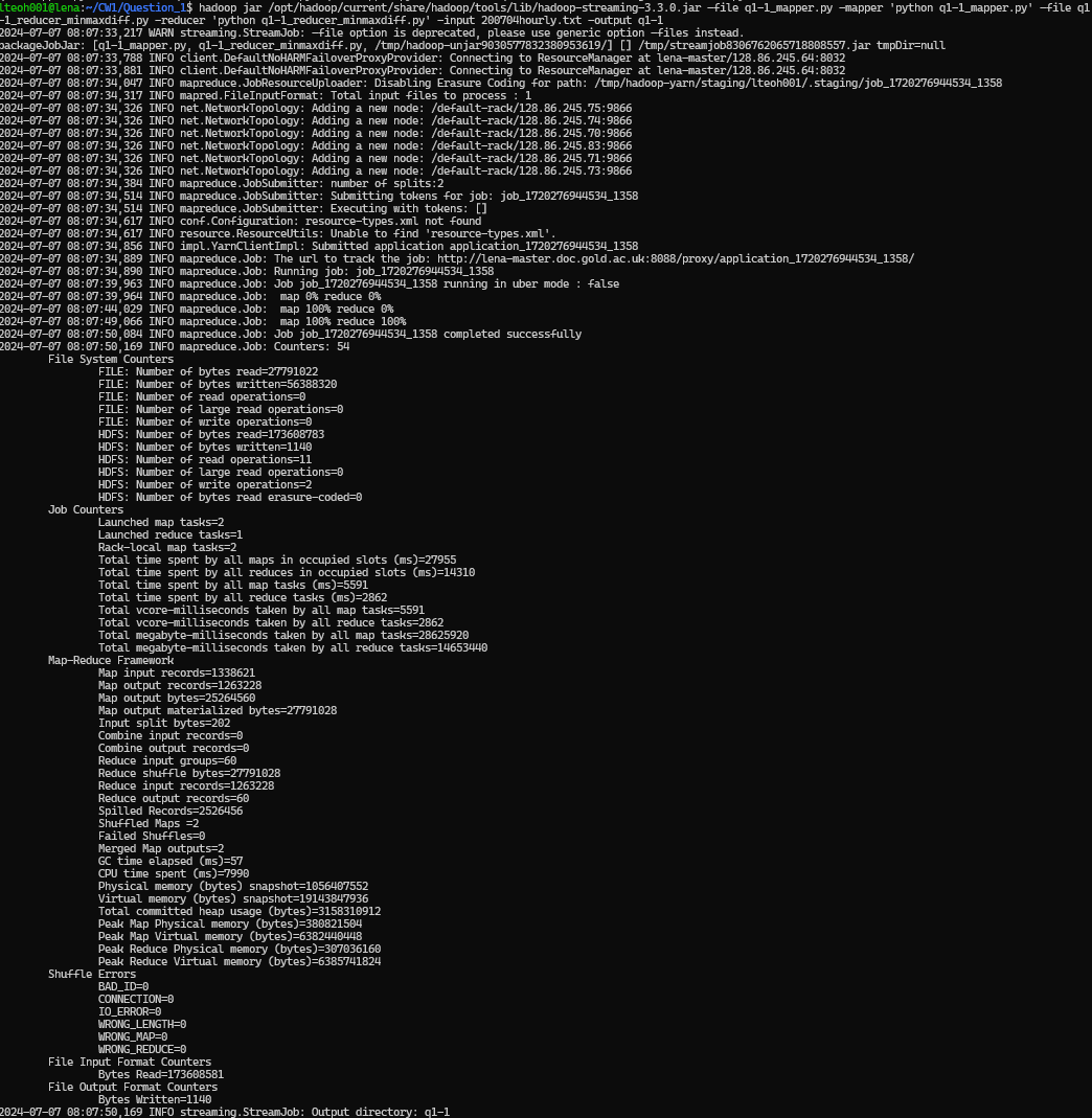

Hadoop Command for Wind Speed Difference

Then extracted the reuslt output folder to local folder, and then pritn the result statement. Using the following commands:

hadoop fs -get q1-1
cd q1-1
cat part-0000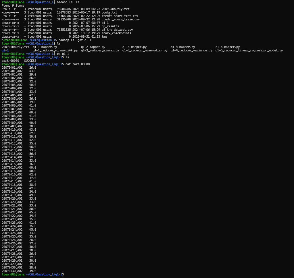

The daily maximum and minimum “Dry Bulb Temp” across all weather stations

Pseudo Code

The Mapper

For each line from the input file
    Remove all spaces adn then split the data where there is a ','
    if dry bulb temp (removing blank/white spaces and removing '-') is a digit
        if station type not '-'
            print date and station type as key, and wind speed as value, pair.

The Reducer

initialize placeholders
datestation
max dry bulb temp
min dry bulb temp

for each line from the input file
    extract the keys and value
    if placeholders have no value
        update the datestation with key, max dry bulb temp and min dry bulb temp with the current dry bulb temp
    else
        if the datestation is the same
            check if min dry bulb temp is larger than current dry bulb temp
                set min dry bulb temp to current dry bulb temp
            check if max dry bulb temp is smaller than current dry bulb temp
                set max dry bulb temp to current dry bulb temp
        else
            output result of previous datestation with the current max dry bulb temp and current min dry bulb temp
            reset placeholder, set datestation with current key, min and max dry bulb temp with current dry bulb temp
output result of current datestation with current max dry bulb temp and current min dry bulb temp

Code

The Mapper

import sys

# Looping through the dataset
for line in sys.stdin:

    # Processing and individualize the data
    data = line.strip().split(",") # Remove the newline and split by ","

    # Based on Initial Analysis of the dataset
    # Column 1 - YearMonthDay
    # Column 3 - Station Type
    # Column 8 - Dry Bulb Temp

    # If Dry Bulb Temp is digit, as the header and "-" are not.
    if data[8].strip().lstrip('-').isdigit():
        if data[3] != "-": # Remove those without station type listed
            # Output the YearMonthDay and Station Type together, and Dry Bulb Temp
            print("%s\t%s" % (f"{data[1]},{data[3]}", data[8]))

The Reducer

import sys

# Initialize placeholder variables
date_station = None
max_dry_bulb_temp = float(0.00)
min_dry_bulb_temp = float(0.00)

# Loop through the sorted input
for line in sys.stdin:
    (keys, value) = line.split('\t')  # Individualizing the input data
    dry_bulb_temp = float(value) # Extract dry bulb temp from value

    # If date_station is empty
    # Initialize the date_station and the placeholders with first input data received
    if date_station == None:
        date_station = keys
        max_dry_bulb_temp = dry_bulb_temp
        min_dry_bulb_temp = dry_bulb_temp

    # If date is not empty
    # Means that the placeholder variables has values to compare with
    elif date_station:

        # If the data_station is the same as current
        if date_station == keys:
            if max_dry_bulb_temp < dry_bulb_temp:
                max_dry_bulb_temp = dry_bulb_temp

            if min_dry_bulb_temp > dry_bulb_temp:
                min_dry_bulb_temp = dry_bulb_temp

        # If the Current date_station is not the same as placeholder Station
        # which shows that the sorted data as move on to another station or day already
        elif date_station != keys:

            # Print current result
            print(date_station + "\t" + str(min_dry_bulb_temp) + "," + str(max_dry_bulb_temp))

            # Reset the placeholder value to the new current values
            date_station = keys
            max_dry_bulb_temp = dry_bulb_temp
            min_dry_bulb_temp = dry_bulb_temp

# Print final result
print(date_station + "\t" + str(min_dry_bulb_temp) + "," + str(max_dry_bulb_temp))

Result

Running the command:

hadoop jar /opt/hadoop/current/share/hadoop/tools/lib/hadoop-streaming-3.3.0.jar \
 -file q1-2_mapper.py -mapper 'python q1-2_mapper.py' \
 -file q1-2_reducer_minmax.py -reducer 'python q1-2_reducer_minmax.py' \
 -input 200704hourly.txt \
 -output q1-2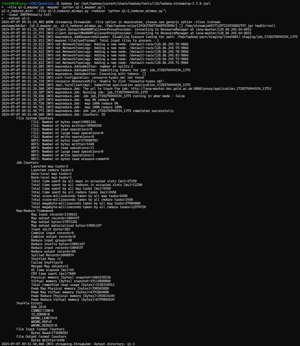

Hadoop Command for Dry Bulb Temp Min/Max

Then extracted the results output folder to local folder, and then print the result statements. Using the following statements.

hadoop fs -get q1-2
cd q1-2
cat part-0000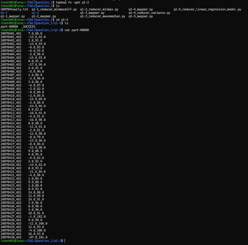

The daily mean and median of 'Dry Bulb Temp' over all weather stations

Pseudo Code

The Mapper

For each line from the input file
    Remove all spaces adn then split the data where there is a ','
    if dry bulb temp (removing blank/white spaces and removing '-') is a digit
        if station type not '-'
            print date and station type as key, and wind speed as value, pair.

The Reducer

Initialize placeholders
datestation
count
total dry bulb temp
dry bulb temp list

for each line from the input file
    extract the keys and values
    if placeholder have no values
        update datestation with key
        count add 1 to itself
        set total dry bulb temp current dry bulb temp
        add current dry bulb temp into the list
    else
        if datestation is the same as the current datestation
            count add 1 to itself
            total dry dulb temp add the current dry bulb temp value to itself
            dry bulb temp list append the current dry bulb temp value into the list

        else datestation is not the same as the current datestaion
            Get the value of median by
                if count is divisible by 2
                    Get the value of ((count/2)-1)th in the dry bulb temp list
                    Get the value of (count/2)th in the dry bulb temp list
                    Get the median value by getting the average of median left and median right
                else
                    Get the value of ((count-1)/2)th value in the dry bulb temp list

            Get the value of mean by dividing the total dry bulb temp value with count.
            Print the previous datestation and current values of mean and median

            Reset the placeholders and set current values
            set datastation to current keys
            set count to 1
            total dry bulb temp to current dry bulb temp
            dry bulb temp list hold only current dry bulb temp

Get the value of median by
    if count is divisible by 2
        Get the value of ((count/2)-1)th in the dry bulb temp list
        Get the value of (count/2)th in the dry bulb temp list
        Get the median value by getting the average of median left and median right
    else
        Get the value of ((count-1)/2)th value in the dry bulb temp list

Get the value of mean by dividing the total dry bulb temp value with count.
Print the previous datestation and current values of mean and median

Code

The Mapper

import sys

# Looping through the dataset
for line in sys.stdin:

    # Processing and individualize the data
    data = line.strip().split(",") # Remove the newline and split by ","

    # Based on Initial Analysis of the dataset
    # Column 1 - YearMonthDay
    # Column 3 - Station Type
    # Column 8 - Dry Bulb Temp

    # If Dry Bulb Temp is digit, as the header and "-" are not.
    if data[8].strip().lstrip('-').isdigit():
        if data[3] != "-": # Remove those without station type listed
            # Output the YearMonthDay and Station Type together, and Dry Bulb Temp
            print("%s\t%s" % (f"{data[1]},{data[3]}", data[8]))

The Reducer

import sys

# Initializing placeholder variables
date_station = None
count = int(0)
total_dry_bulb_temp = float(0.00)
dry_bulb_temp_list = []

# Looping through the sorted input
for line in sys.stdin:
    (keys, value) = line.split('\t')
    dry_bulb_temp = float(value)

    # If date_station is empty
    if date_station == None:
        date_station = keys
        count = 1
        total_dry_bulb_temp = dry_bulb_temp
        dry_bulb_temp_list = [dry_bulb_temp]

    # If datastattion has value
    elif date_station:

        # If datestation is the same as the current datestation
        if date_station == keys:

            # Update placeholders accordingly
            count += 1
            total_dry_bulb_temp += dry_bulb_temp
            dry_bulb_temp_list.append(dry_bulb_temp)

        # If datestation is not the same as the current datestation
        elif date_station != keys:

            # Getting the Median value
            # Sort the dry bulb temp list
            dry_bulb_temp_list = sorted(dry_bulb_temp_list)

            # If the current count is divisible by two
            if count % 2 == 0:

                # Get the value of ((count/2)-1)th in the dry bulb temp list
                median_left = float(dry_bulb_temp_list[int(count/2-1)])

                # Get the value of (count/2)th in the dry bulb temp list
                median_right = float(dry_bulb_temp_list[int(count/2)])

                # Get the median value by getting the average of median left and median right
                median = (median_left + median_right) / 2

            # If the current count is not divisible by two
            elif count % 2 != 0:
                median = dry_bulb_temp_list[int((count-1)/2)]

            # Getting the Mean value
            mean = total_dry_bulb_temp / count

            # Print the results, the previous datestation and the mean and median
            print(date_station + "\t" + str(mean) + "," + str(median))

            # Reset the placeholders and set current values
            date_station = keys
            count = 1
            total_dry_bulb_temp = dry_bulb_temp
            dry_bulb_temp_list = [dry_bulb_temp]

# Getting the Median value
dry_bulb_temp_list = sorted(dry_bulb_temp_list)
if count % 2 == 0:
    median_left = float(dry_bulb_temp_list[int(count/2-1)])
    median_right = float(dry_bulb_temp_list[int(count/2)])
    median = (median_left + median_right) / 2

elif count % 2 != 0:
    median = dry_bulb_temp_list[int((count-1)/2)]

# Getting the mean value
mean = total_dry_bulb_temp / count

# Print the results, the previous datestation and the mean and median
print(date_station + "\t" + str(mean) + "," + str(median))

Result

Running the following command:

hadoop jar /opt/hadoop/current/share/hadoop/tools/lib/hadoop-streaming-3.3.0.jar \
 -file q1-3_mapper.py -mapper 'python q1-3_mapper.py' \
 -file q1-3_reducer_meanmedian.py -reducer 'python q1-3_reducer_meanmedian.py' \
 -input 200704hourly.txt \
 -output q1-3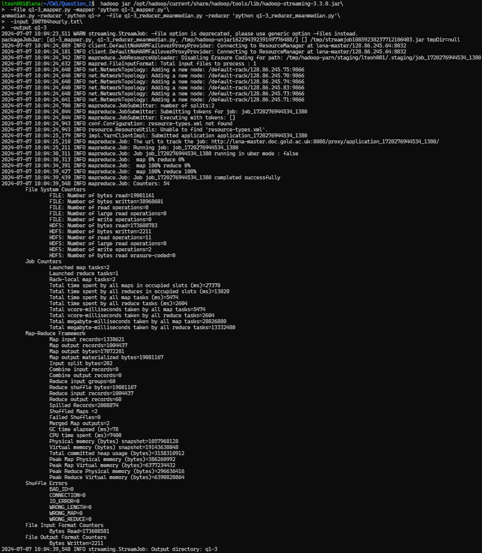

Hadoop Command for Dry Bulb Temp Mean/Median

Then extracted the results output folder to local folder, and then print the result statements. Using the following commands.

hadoop fs -get q1-3
cd q1-3
cat part-0000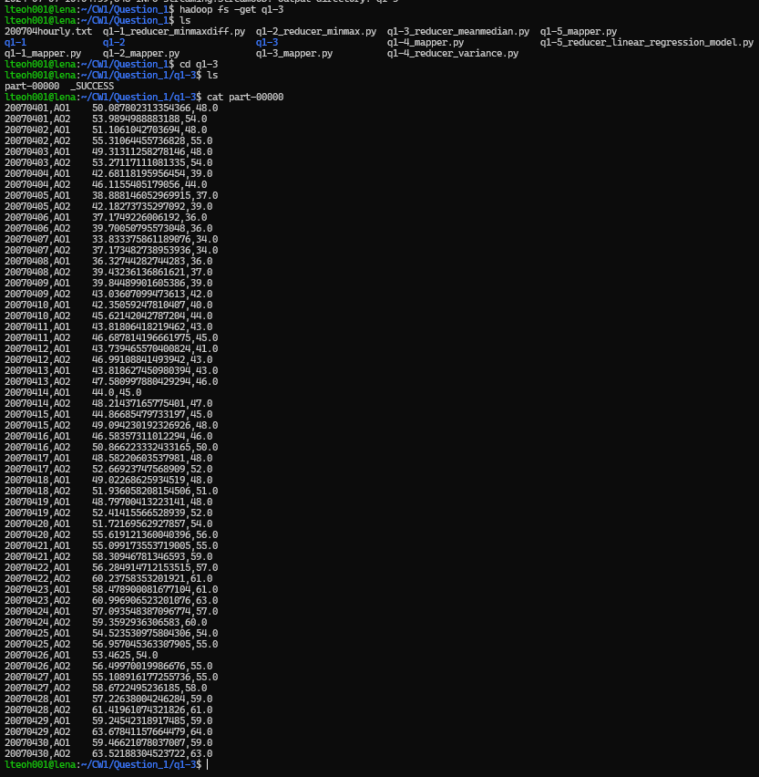

The daily variance of 'Dry Bulb Temp' over all weather stations

The following are the pseudo code.

Pseudo Code

The Mapper

For each line from the input file
    Remove all spaces adn then split the data where there is a ','
    if dry bulb temp (removing blank/white spaces and removing '-') is a digit
        if station type not '-'
            print date and station type as key, and wind speed as value, pair.

The Reducer

Initialize placeholder
datestation
dry bulb temp square total
dry bulb temp total
count
variance

for each line from the mapper
    extract key and value

    if datestation is empty
        set the placeholder values
        set datestation as current key
        dry bulb temp square total = current dry bulb temp square
        dry bulb temp total = dry bulb temp square
        count

    else if datestation is not empty
        if datestation is the same as current key
            count add 1 to itself
            dry bulb temp total add the current dry bulb temp to itself
            dry bulb temp square add the square of current dry bulb temp to itself

        else
            get the mean value by dividing the dry bulb temp total divided by count
            get the variance by the equation set in the coursework specs (dry bulb temp square_total - (count*(mean**2))) / count
            print the datestation and the results of mean and variance

            reset the placeholders
            set datestation to current key
            set count to 1
            set dry bulb temp total to current dry bulb temp
            set dry bulb temp square total to current dry bulb temp square

get the mean value by dividing the dry bulb temp total divided by count
get the variance by the equation set in the coursework specs (dry bulb temp square_total - (count*(mean**2))) / count
print the datestation and the results of mean and variance

Code

The Mapper

import sys

# Looping through the dataset
for line in sys.stdin:

    # Processing and individualize the data
    data = line.strip().split(",") # Remove the newline and split by ","

    # Based on Initial Analysis of the dataset
    # Column 1 - YearMonthDay
    # Column 3 - Station Type
    # Column 8 - Dry Bulb Temp

    # If Dry Bulb Temp is digit, as the header and "-" are not.
    if data[8].strip().lstrip('-').isdigit():
        if data[3] != "-": # Remove those without station type listed
            # Output the YearMonthDay and Station Type together, and Dry Bulb Temp
            print("%s\t%s" % (f"{data[1]},{data[3]}", data[8]))

The Reducer

import sys

# Initialize the placeholders
date_station = None
dry_bulb_temp_square_total = float(0)
dry_bulb_temp_total = float(0)
count = 0
variance = float(0)

# Loop through the values from mapper
for line in sys.stdin:

    # Extract the keys and values
    (keys, value) = line.split('\t')
    dry_bulb_temp = float(value)

    # If datastation is empty
    if date_station == None:

        # Set the placeholders with current value
        date_station = keys
        dry_bulb_temp = float(value)
        count = 1
        dry_bulb_temp_total = dry_bulb_temp
        dry_bulb_temp_square_total = dry_bulb_temp ** 2

    # If the datestation not empty
    elif date_station:

        # If the datestation and key has same values
        if date_station == keys:

            # Update the placeholders
            count += 1
            dry_bulb_temp_total += dry_bulb_temp
            dry_bulb_temp_square_total += dry_bulb_temp ** 2

        # If the datestation and key are not the same
        elif date_station != keys:

            # Get the mean
            mean = dry_bulb_temp_total / count

            # Get the variance
            variance = (dry_bulb_temp_square_total - (count*(mean**2))) / count

            # Print the previous datestation, mean and variance
            print(date_station + '\t' + str(variance))

            # Reset the placeholders
            date_station = keys
            dry_bulb_temp = float(value)
            count = 1
            dry_bulb_temp_total = dry_bulb_temp
            dry_bulb_temp_square_total = dry_bulb_temp ** 2

# Get the mean
mean = dry_bulb_temp_total / count

# Get the variance
variance = (dry_bulb_temp_square_total - (count*(mean**2))) / count

# Print the previous datestation, mean and variance
print(date_station + '\t' + str(variance))

Result

Running the following command:

hadoop jar /opt/hadoop/current/share/hadoop/tools/lib/hadoop-streaming-3.3.0.jar \
 -file q1-4_mapper.py -mapper 'python q1-4_mapper.py' \
 -file q1-4_reducer_variance.py -reducer 'python q1-4_reducer_variance.py' \
 -input 200704hourly.txt \
 -output q1-4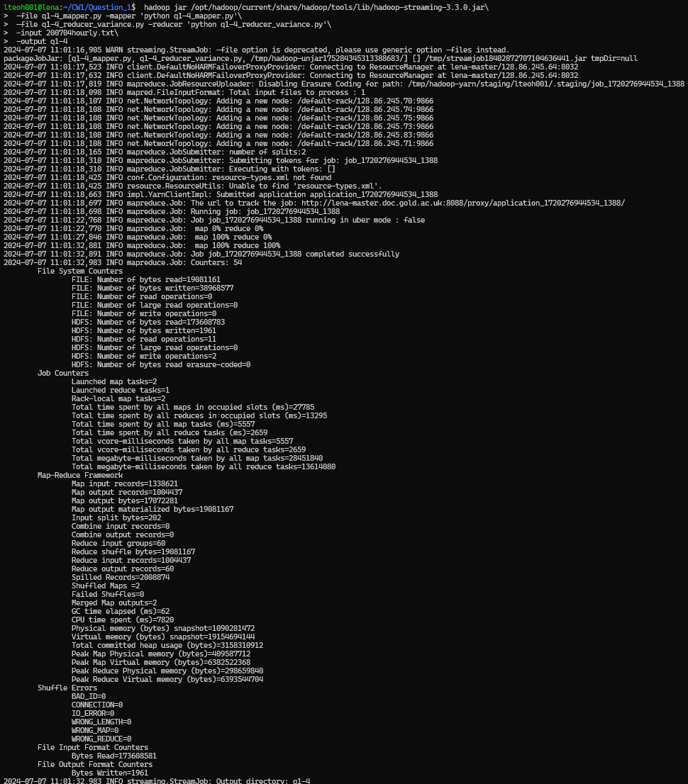

Hadoop Command for Dry Bulb Temp Variance

Then extracted the results output folder to local folder, and then print the result statements. Using the following command.

hadoop fs -get q1-4
cd q1-4
cat part-0000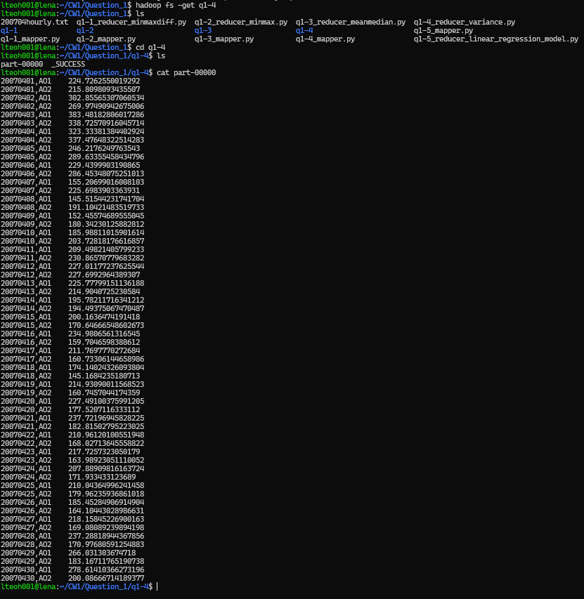

Develop MapReduce jobs to perform linear regression analysis on the weather data set, fitting a linear model to the data of any two variables of your choice

The following are the pseudo code.

Pseudo Code

The Mapper

For each line from the input file
    Remove all spaces and then split the data where there is a ','
    if Dry Bulb Temp and Wind Speed (after removing blank/white spaces and removing '-') is a digit
        if station type is not '-'
            print a constant as key, and dry bulb temp and wind speed as a tuple value, as a pair

The Reducer

initialize placeholders
count
sumxy
sumx
sumy
sumxsquare

for each line from input file
    extract the key and value
    the value can then be split into x and y

    count add 1 to itself
    sumxy add x * y to itself
    sum_x add x to itself
    sum_y add y to itself
    sum_x_square add x ** 2 to itself

slope = ((count * sumxy) - (sumx * sumy) ) / ((count * sumxsquare) - (sumx ** 2))
intercept = (sumy - (slope * sumx)) / count

print result of the slope and intercept

Code

The Mapper

import sys

# Looping through the dataset
for line in sys.stdin:

    # Processing and individualize the data
    data = line.strip().split(",") # Remove the newline and split by ","

    # Based on Initial Analysis of the dataset
    # Column 8 - Dry Bulb Temp
    # Column 12 - Wind Speed

    # If Dry Bulb Temp and Wind Speed are digit, as the header and "-" are not.
    if data[8].strip().lstrip('-').isdigit() and data[12].strip().lstrip('-').isdigit():
        if data[3] != "-": # Remove those without station type listed
            # Output the YearMonthDay, and Dry Bulb Temp with Wind Speed together.
            print("%s\t%s" % ('A', f"{data[8]},{data[12]}"))

The Reducer

import sys

# m = (n sum(xy) - sum(x)sum(y)) / (n sum(x^2) - sum(x)^2)
# b = sum(y) - m sum(x) / n

count = int(0)
sum_xy = float(0)
sum_x = float(0)
sum_y = float(0)
sum_x_square = float(0)


for line in sys.stdin:

    (keys, value) = line.split('\t')
    x, y = value.split(',')
    x = float(x)
    y = float(y)

    count += 1
    sum_xy += x * y
    sum_x += x
    sum_y += y
    sum_x_square += x ** 2

slope = ((count * sum_xy) - (sum_x * sum_y) ) / ((count * sum_x_square) - (sum_x ** 2))
intercept = (sum_y - (slope * sum_x)) / count

print(str(slope) + ", " + str(intercept))

Result

Running the following command:

hadoop jar /opt/hadoop/current/share/hadoop/tools/lib/hadoop-streaming-3.3.0.jar \
 -file q1-5_mapper.py -mapper 'python q1-5_mapper.py' \
 -file q1-5_reducer_linear_regression_model.py -reducer 'python q1-5_reducer_linear_regression_model.py' \
 -input 200704hourly.txt \
 -output q1-5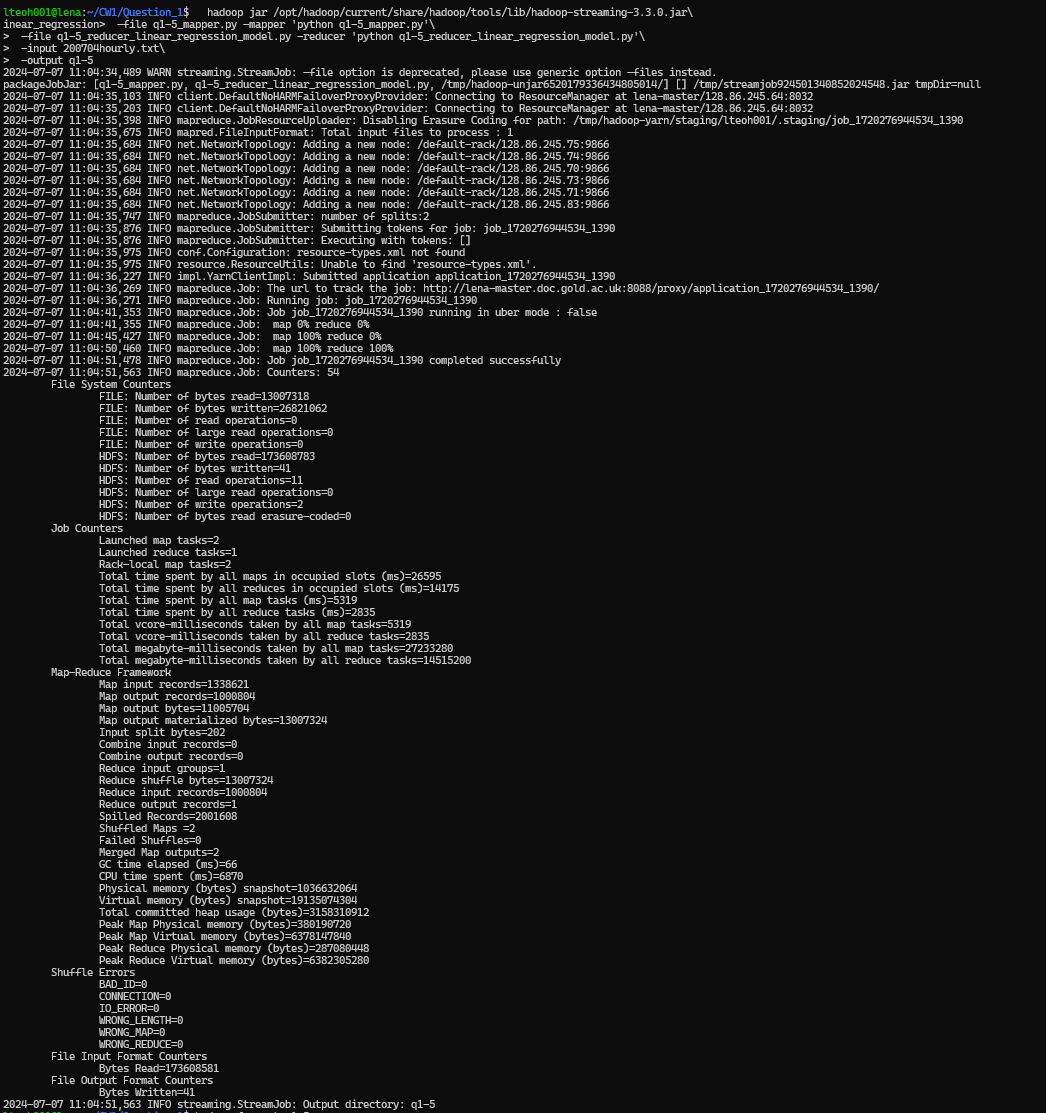

Then extracted the results output folder to local folder, and then print the result statements. Using the following commands.

hadoop fs -get q1-5
cd q1-5
cat part-0000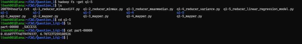

Question 2 – Cluster Analysis using Apache Mahout

Following university study materials, we performed K-means clustering using Euclidean and Manhattan distance measures on the "French Plays" dataset. The following are the steps taken to run it, with the accompanying screenshots.

Creating Folder

Firstly, we use the make a folder for the dataset to be stored, using the following commands:

hadoop fs -mkdir ./docs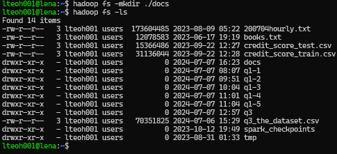

Upload Dataset

The dataset that has been chosen is the french plays, which is also obtained from the UOL portal. Using the following commands, we were able to upload them to the HDFS environment.

hadoop fs -copyFromLocal ./french-plays/* ./docs/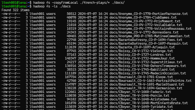

Creating Sequences

We then create sequence files form the raw text using the following commands:

mahout seqdirectory -i docs -o docs-seqfiles -c UTF-8 -chunk 5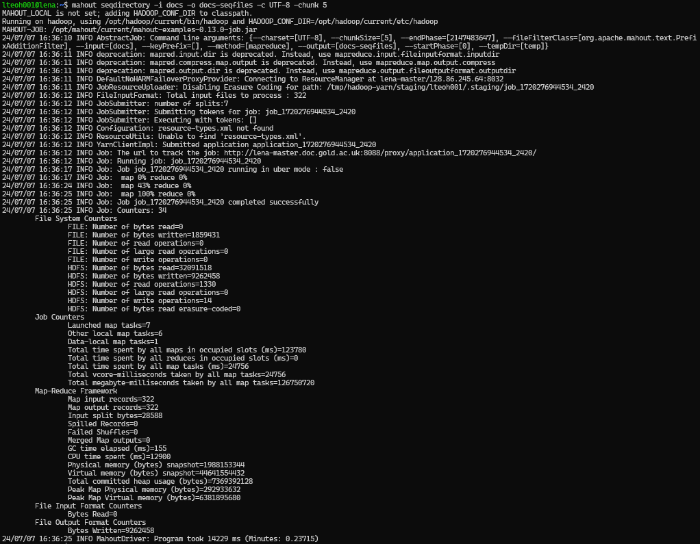

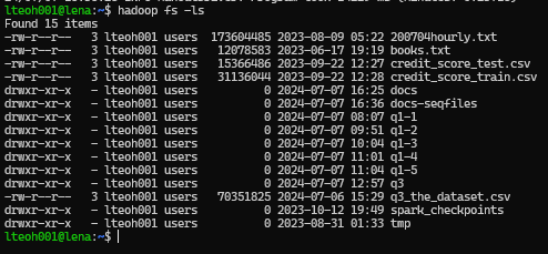
As shown in the following screenshot, where the docs-seqfiles folder is created:

Creating Sparse Representation

Then, we create a sparse representation of the vectors with the following command:

mahout seq2sparse -nv -i docs-seqfiles -o docs-vectors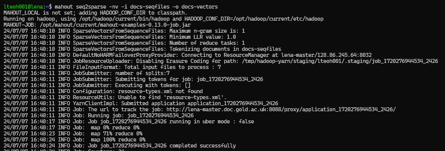

Creating Canopies

We then created the canopies, which need to be created for the Euclidean and Manhattan distance measures. Therefore, running this two times with the following commands:

mahout canopy -i docs-vectors/tfidf-vectors -ow -o docs-vectors/docs-canopy-centroids-ed -dm org.apache.mahout.common.distance.EuclideanDistanceMeasure -t1 0.5 -t2 0.3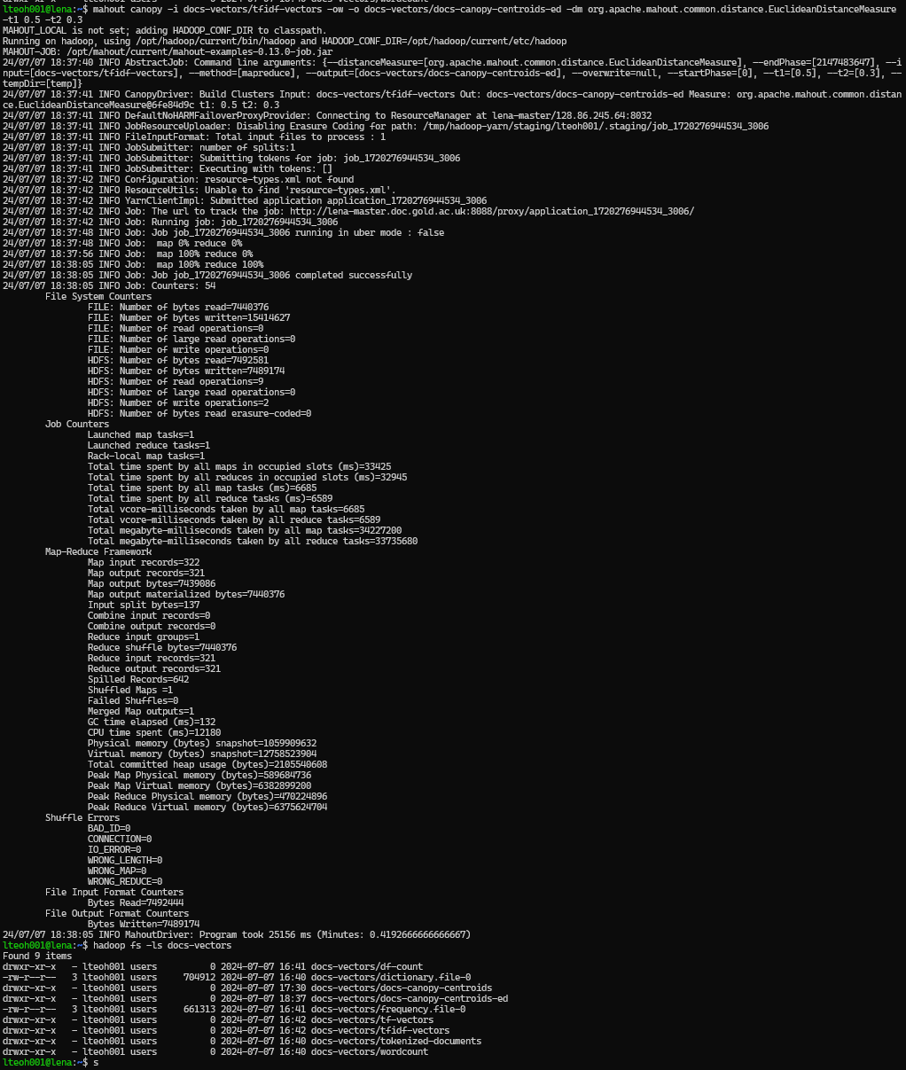

mahout canopy -i docs-vectors/tfidf-vectors -ow -o docs-vectors/docs-canopy-centroids-md -dm org.apache.mahout.common.distance.ManhattanDistanceMeasure -t1 0.5 -t2 0.3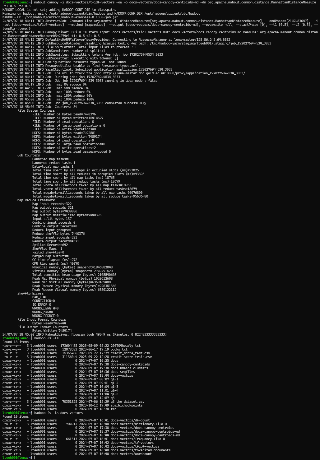

Running K-Means

Euclidean Distance

Now, we are ready to run the kmean clustering accordingly. We have selected to perform with k = 5 until 25, with a 5 step increment, using the following commands:

for k in {5..25..5}
do
mahout kmeans -i docs-vectors/tfidf-vectors -c docs-canopy-centroids-ed -o hdfs://lena/user/lteoh001/docs-kmeans-clusters-euclidean$k -dm org.apache.mahout.common.distance.EuclideanDistanceMeasure -cl -cd 0.1 -ow -x 20 -k $k
done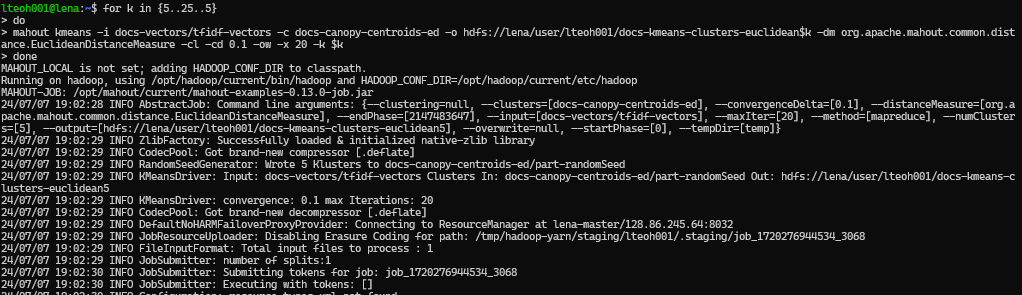

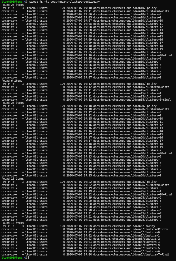
Which will result having the following output folders:

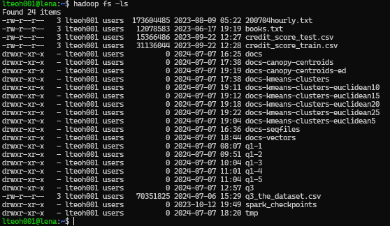
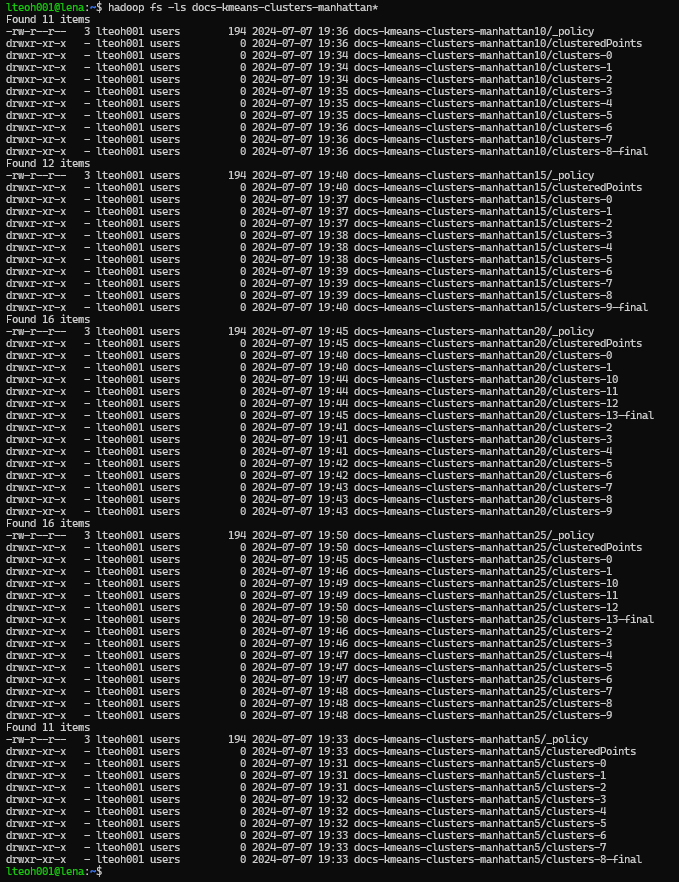
Manhattan Distance

The following command is the same as above but for Manhattan Distance. However there is no screenshot for the running of the command. But the screenshot shown is the result of running the command, where all the output folder can be seen.

for k in {5..25..5}
do
mahout kmeans -i docs-vectors/tfidf-vectors -c docs-canopy-centroids-md  -o hdfs://lena/user/lteoh001/docs-kmeans-clusters-manhattan$k -dm org.apache.mahout.common.distance.ManhattanDistanceMeasure -cl -cd 0.1 -ow -x 20 -k $k
done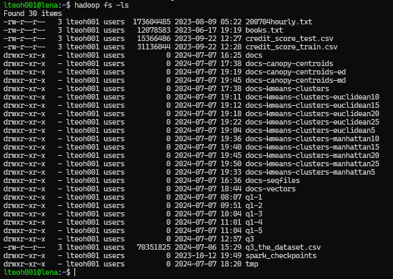

Evaluation

Then, we using the following command to get the results, with some changes to -i, -o and -p according to the number of k.

mahout clusterdump -dt sequencefile -d docs-vectors/dictionary.file-* -i docs-kmeans-clusters-euclidean5/clusters-7-final -o clusters-euclidean5.txt -b 100 -p docs-kmeans-clusters-euclidean5/clusteredPoints -n 20 --evaluate

The following screenshot is what we need to look into, and then finding the one that states 'final'. Then, that is the folder then we want to direct to and access it for evaluation. One is for Euclidean and one is for Manhattan.

We had to painstakingly look into all the cluster output folder, and look for the final one to be used. When using the following command, it did not work for some reason. I might be doing it wrong, so we ended up getting the values of the final folder one by one, and generate the output one by one.

mahout clusterdump -dt sequencefile -d docs-vectors/dictionary.file-* -i docs-kmeans-clusters/clusters-*-final -o clusters.txt -b 100 -p docs-kmeans-clusters/clusteredPoints -n 20 --evaluate

As we wanted to make it into a simpler process of using the following, but somehow the part on -i docs-kmeans-clusters/clusters-*-final did not work. Hence, we needed to run every evaluation line.

for i in {5..25..5}
do
mahout clusterdump -dt sequencefile -d docs-vectors/dictionary.file-* -i docs-kmeans-clusters-euclidean$i/*-final -o cluster-euclidean$i.txt -b 100 -p docs-kmeans-clusters-euclidean$i/clusteredPoints -dm org.apache.mahout.common.distance.EuclideanDistanceMeasure -n 20 --evaluate
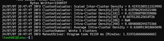
done

The following is the how the result will show. We will be taking the inter cluster density and intra-cluster density. This is the results when it is finish running.

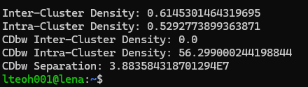
The following is the result when we open the text according to the following command.

The following are the results from running k-means with k = 5 until 25.

Distance Measure	k	Inter-Cluster Density	Intra-Cluster Density
Euclidean	5	0.447506	0.629493
Euclidean	10	0.496821	0.601571
Euclidean	15	0.63299	0.668097
Euclidean	20	0.535608	0.498665
Euclidean	25	0.554156	0.574811
Manhattan	5	0.419315	0.626091
Manhattan	10	0.411877	0.601849
Manhattan	15	0.249065	0.597199
Manhattan	20	0.41641	0.598346
Manhattan	25	0.353692	0.483333

We also have recorded the results into an excel file which we can just extract to python for data visualization.

# Importing libraries
from matplotlib import pyplot as plt
import numpy as np
import pandas as pd

# Extracting the excel file
results = pd.read_excel('results.xlsx')
results.columns

Index(['Distance Measure', 'k', 'Inter-Cluster Density',
       'Intra-Cluster Density'],
      dtype='object')

# Filter only those that are for euclidean distance
euclidean = results[results['Distance Measure'] == 'Euclidean']

# Plotting Inter Cluster
plt.plot(euclidean[euclidean['k'] < 30]['k'], euclidean[euclidean['k'] < 30]['Inter-Cluster Density'])
plt.title('Inter-Cluster Density')
plt.show()

# Plotting Intra Cluster
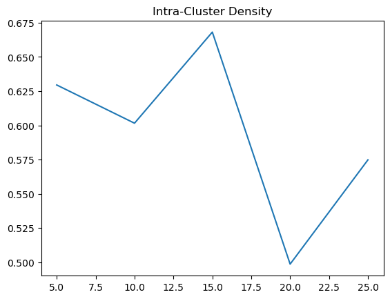
plt.plot(euclidean[euclidean['k'] < 30]['k'], euclidean[euclidean['k'] < 30]['Intra-Cluster Density'])
plt.title('Intra-Cluster Density')
plt.show()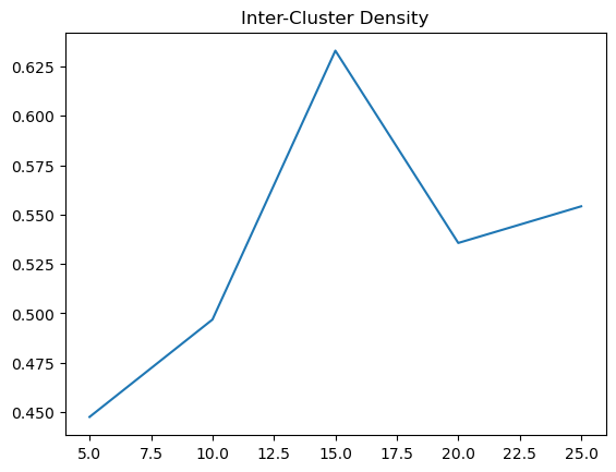

# Filter those that are Manhattan
manhattan = results[results['Distance Measure'] == 'Manhattan']

# Plotting Inter Cluster
plt.plot(manhattan[manhattan['k'] < 30]['k'], manhattan[manhattan['k'] < 30]['Inter-Cluster Density'])
plt.title('Inter-Cluster Density')
plt.show()

# Plotting Intra Cluster
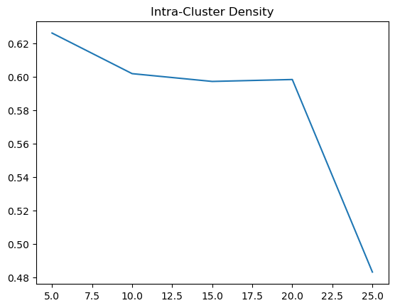
plt.plot(manhattan[manhattan['k'] < 30]['k'], manhattan[manhattan['k'] < 30]['Intra-Cluster Density'])
plt.title('Intra-Cluster Density')
plt.show()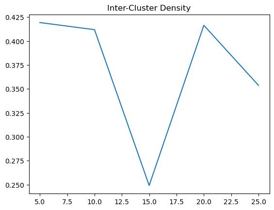

Running it again, at K = 30 to 70

After graphing plotting, we realized that we might need more runs with the number of k to see if a more obvious trend can be observed. We are to expect the inter-cluster distance to increase when k increase, because there should be more distinctive groups, and for intra-cluster, we expect to grow smaller over time as k increase because there should be more data points that should be similar to one another.

We run the same command as above, but for k = 30 to 70 at a 10 step increment. Using the following commands.

for k in {30..70..10}
do
mahout kmeans -i docs-vectors/tfidf-vectors -c docs-canopy-centroids-ed -o hdfs://lena/user/lteoh001/docs-kmeans-clusters-euclidean$k -dm org.apache.mahout.common.distance.EuclideanDistanceMeasure -cl -cd 0.1 -ow -x 20 -k $k
done

for k in {30..70..10}
do
mahout kmeans -i docs-vectors/tfidf-vectors -c docs-canopy-centroids-md -o hdfs://lena/user/lteoh001/docs-kmeans-clusters-manhattan$k -dm org.apache.mahout.common.distance.ManhattanDistanceMeasure -cl -cd 0.1 -ow -x 20 -k $k
done

Then, similarly, we extract it with the same commands where we read the final output file that is stored locally. We also have updated it into the excel and we can quickly use it for data visualization.

Results and Evaluation

The following is the complete table

Distance Measure	k	Inter-Cluster Density	Intra-Cluster Density
Euclidean	5	0.447506	0.629493
Euclidean	10	0.496821	0.601571
Euclidean	15	0.63299	0.668097
Euclidean	20	0.535608	0.498665
Euclidean	25	0.554156	0.574811
Manhattan	5	0.419315	0.626091
Manhattan	10	0.411877	0.601849
Manhattan	15	0.249065	0.597199
Manhattan	20	0.41641	0.598346
Manhattan	25	0.353692	0.483333
Euclidean	30	0.61453	0.529277
Euclidean	40	0.528083	0.562806
Euclidean	50	0.498798	0.575325
Euclidean	60	0.398241	0.554493
Euclidean	70	0.460521	0.555504
Manhattan	30	0.431708	0.583179
Manhattan	40	0.383707	0.588104
Manhattan	50	0.442734	0.574998
Manhattan	60	0.316057	0.586231
Manhattan	70	0.454744	0.66881

# Filter only those that are for euclidean distance
euclidean = results[results['Distance Measure'] == 'Euclidean']

# Plotting Inter Cluster
plt.plot(euclidean['k'], euclidean['Inter-Cluster Density'])
plt.title('Inter-Cluster Density')
plt.show()

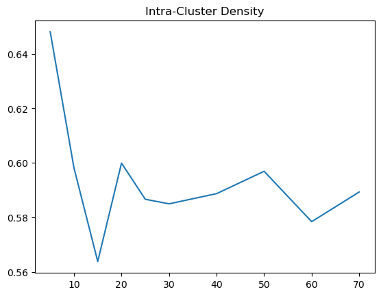
# Plotting Intra Cluster
plt.plot(euclidean['k'], euclidean['Intra-Cluster Density'])
plt.title('Intra-Cluster Density')
plt.show()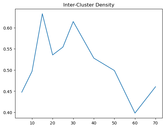

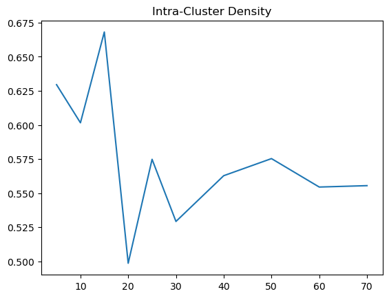
Based on the results, there is a bit of a trend that we can observed. When using Euclidean Distance, the inter cluster density is best at around 15 to 30, where the cluster distinctions are at its highest. However, for the intra cluster density, we can see that it sharply decreases at 20 and climbs back to a baseline. Therefore, using Euclidean distance, the optimal k should be around 20 to 30, where the inter cluster is at its highest and the intra cluster density is at its lowest.

# Filter those that are Manhattan
manhattan = results[results['Distance Measure'] == 'Manhattan']

# Plotting Inter Cluster
plt.plot(manhattan['k'], manhattan['Inter-Cluster Density'])
plt.title('Inter-Cluster Density')
plt.show()

# Plotting Intra Cluster
plt.plot(manhattan['k'], manhattan['Intra-Cluster Density'])
plt.title('Intra-Cluster Density')
plt.show()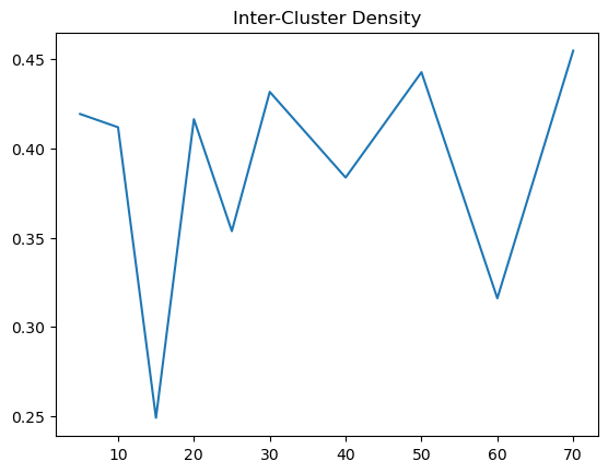

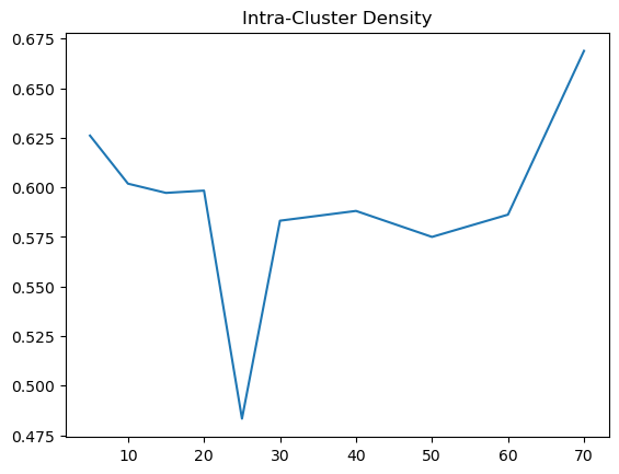
As for using Manhattan distance measure, the trends on our inter cluster density is not as clear as the Euclidean distance measure. It is generally around 0.4, with a peak at 15. However, for the intra cluster density, we can see that it is generally around 0.6, with a peak at 70. Therefore, using Manhattan distance measure, the optimal k should be around 15 to 70, where the inter cluster is at its highest and the intra cluster density is at its lowest.

Repeating the steps above for Cosine

We will now repeat the steps above, but for cosine, and we will do the same analysis again.

Performing K-means

for k in {5..25..5}
do
mahout kmeans -i docs-vectors/tfidf-vectors -c docs-canopy-centroids-md -o hdfs://lena/user/lteoh001/docs-kmeans-clusters-manhattan$k -dm org.apache.mahout.common.distance.ManhattanDistanceMeasure -cl -cd 0.1 -ow -x 20 -k $k
done

for k in {30..70..10}
do
mahout kmeans -i docs-vectors/tfidf-vectors -c docs-canopy-centroids-md -o hdfs://lena/user/lteoh001/docs-kmeans-clusters-manhattan$k -dm org.apache.mahout.common.distance.ManhattanDistanceMeasure -cl -cd 0.1 -ow -x 20 -k $k
done

Evaluate and get result

for k in {5..25..5}
do
mahout clusterdump -dt sequencefile -d docs-vectors/dictionary.file-* -i docs-kmeans-clusters-cosine$k/clusters-2-final -o clusters-consine$k.txt -b 100 -p docs-kmeans-clusters-cosine$k/clusteredPoints -n 20 --evaluate
done

for k in {30..70..10}
do
mahout clusterdump -dt sequencefile -d docs-vectors/dictionary.file-* -i docs-kmeans-clusters-cosine$k/clusters-2-final -o clusters-consine$k.txt -b 100 -p docs-kmeans-clusters-cosine$k/clusteredPoints -n 20 --evaluate
done

We can use a loop this time, because all of them had the 2nd cluster folder as the final folder. Making the extraction easier.

Printing the results

Using the following, we can print out the entire result list, then we will update it accordingly.

tail -n 6 *consine*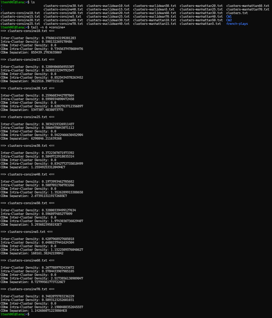

Do not mind the typo, it is supposed to be cosine, but it is mispelled as 'consine'

The following are the result in table. Next, we will plot it and see how it compares to the other distance measures.

Distance Measure	k	Inter-Cluster Density	Intra-Cluster Density
Euclidean	5	0.447506	0.629493
Euclidean	10	0.496821	0.601571
Euclidean	15	0.63299	0.668097
Euclidean	20	0.535608	0.498665
Euclidean	25	0.554156	0.574811
Manhattan	5	0.419315	0.626091
Manhattan	10	0.411877	0.601849
Manhattan	15	0.249065	0.597199
Manhattan	20	0.41641	0.598346
Manhattan	25	0.353692	0.483333
Euclidean	30	0.61453	0.529277
Euclidean	40	0.528083	0.562806
Euclidean	50	0.498798	0.575325
Euclidean	60	0.398241	0.554493
Euclidean	70	0.460521	0.555504
Manhattan	30	0.431708	0.583179
Manhattan	40	0.383707	0.588104
Manhattan	50	0.442734	0.574998
Manhattan	60	0.316057	0.586231
Manhattan	70	0.454744	0.66881
Cosine	5	0.420796	0.648024
Cosine	10	0.376861	0.598132
Cosine	15	0.320841	0.563853
Cosine	20	0.259668	0.599893
Cosine	25	0.303422	0.586647
Cosine	30	0.372237	0.584972
Cosine	40	0.197399	0.588705
Cosine	50	0.328003	0.596897
Cosine	60	0.267789	0.578443
Cosine	70	0.348288	0.589312

Evaluate and Visualize

# Filter those that are Manhattan
Cosine = results[results['Distance Measure'] == 'Cosine']

# Plotting Inter Cluster
plt.plot(Cosine['k'], Cosine['Inter-Cluster Density'])
plt.title('Inter-Cluster Density')
plt.show()

# Plotting Intra Cluster
plt.plot(Cosine['k'], Cosine['Intra-Cluster Density'])
plt.title('Intra-Cluster Density')
plt.show()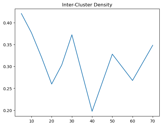

Based on the results, we can see that the inter cluster density for cosine is more like a U shape, which makes deciding the optimal K. Given that inter cluster density is not an obvious choice to pick, we can observe intra cluster density first. For intra, we noted that there is a big drop, resembling an elbow and then it hovers at a range of .58 to .6. Therefore, the optimal k from intra would be 15 and beyond. But because we might want to have a higher inter cluster density, around k = 25 to 30 would be good.

Cluster Analysis

# Getting the average value from all the k value
results.groupby('Distance Measure').mean()[['Inter-Cluster Density', 'Intra-Cluster Density']].sort_values('Inter-Cluster Density')

	Inter-Cluster Density	Intra-Cluster Density
Cosine	0.319530	0.593488
Manhattan	0.387931	0.590814
Euclidean	0.516725	0.575004

Because we would like the value of inter cluster to be higher, while intra cluster to be lower. If we were to have a number inter-cluster divided by intra cluster, we can see which number of k and distance measure performs best.

# Getting the 'optimal' determined by our observations
results['Inter-Cluster over Intra-Cluster'] = results['Inter-Cluster Density'] / results['Intra-Cluster Density']
results.sort_values('Inter-Cluster over Intra-Cluster', ascending=False)

Distance Measure	k	Inter-Cluster Density	Intra-Cluster Density	Inter-Cluster over Intra-Cluster
Euclidean	30	0.614530	0.529277	1.161074
Euclidean	20	0.535608	0.498665	1.074084
Euclidean	25	0.554156	0.574811	0.964066
Euclidean	15	0.632990	0.668097	0.947452
Euclidean	40	0.528083	0.562806	0.938304
Euclidean	50	0.498798	0.575325	0.866985
Euclidean	70	0.460521	0.555504	0.829015
Euclidean	10	0.496821	0.601571	0.825873
Manhattan	50	0.442734	0.574998	0.769975
Manhattan	30	0.431708	0.583179	0.740267
Manhattan	25	0.353692	0.483333	0.731777
Euclidean	60	0.398241	0.554493	0.718207
Euclidean	5	0.447506	0.629493	0.710899
Manhattan	20	0.416410	0.598346	0.695935
Manhattan	10	0.411877	0.601849	0.684353
Manhattan	70	0.454744	0.668810	0.679930
Manhattan	5	0.419315	0.626091	0.669735
Manhattan	40	0.383707	0.588104	0.652448
Cosine	5	0.420796	0.648024	0.649352
Cosine	30	0.372237	0.584972	0.636333
Cosine	10	0.376861	0.598132	0.630063
Cosine	70	0.348288	0.589312	0.591008
Cosine	15	0.320841	0.563853	0.569015
Cosine	50	0.328003	0.596897	0.549514
Manhattan	60	0.316057	0.586231	0.539134
Cosine	25	0.303422	0.586647	0.517214
Cosine	60	0.267789	0.578443	0.462948
Cosine	20	0.259668	0.599893	0.432857
Manhattan	15	0.249065	0.597199	0.417055
Cosine	40	0.197399	0.588705	0.335311

Comparison with the other methods

The thing that were noted when running all three distance measure with Kmeans, cosine performed the fastest and it had very little cluster outputs, as compared to the other 2.

However, when we use our criteria to evaluate, using the Inter-cluster to divide over intra cluster, we can see that Euclidean performs best overall, as well as best at 20 to 30, as mentioned above. For Manhattan, we mentioned also it would be best around 20 to 30, especially 25, but 50 surprisingly was a better choice by a small margin, and Cosine performed worst compare to the others overall and its best performing k were 5, 30 and 10, which was not near to our estimate.

Question 3 - Use a classifier to distinguish between cats and dogs

The Mapper

import sys

# Looping through the input
for line_no, line in enumerate(sys.stdin):

    # Check if the line is not the header
    if line_no > 0:

        # Strip leading/trailing spaces and split by commas
        data = line.strip().split(",")

        # Ensure there are at least two columns
        if len(data) >= 2:

            print('%s\t%s' % (data[0], data[1]))

The Reducer

import os
# Set the cache directory for Hugging Face model
os.environ['HF_HOME'] = '.cache'

import sys
import io
import torch
import base64
from PIL import Image
import open_clip

# Helper function to find the index of the maximum value in an iterable
def argmax(iterable):
    return max(enumerate(iterable), key=lambda x: x[1])[0]

# Initialize the pre-trained model and tokenizer
model, preprocess = open_clip.create_model_from_pretrained('hf-hub:laion/CLIP-ViT-g-14-laion2B-s12B-b42K')
tokenizer = open_clip.get_tokenizer('hf-hub:laion/CLIP-ViT-g-14-laion2B-s12B-b42K')

class_names = ["a dog", "a cat"]
text = tokenizer(class_names)

# Read input lines from the standard input
for line in sys.stdin:

    # Split the line into image name and image data
    image_name, image_data = line.strip().split('\t')

    # Decode the base64 encoded image data and open it as a PIL image
    image = Image.open(
        io.BytesIO(
            base64.decodebytes(bytes(image_data, "utf-8"))
        )
    )

    # Preprocess the image for the CLIP model
    image = preprocess(image).unsqueeze(0)

    # Perform inference with the model without calculating gradients (for efficiency)
    with torch.no_grad(), torch.cuda.amp.autocast():

        # Encode the image and text using the CLIP model
        image_features = model.encode_image(image)
        text_features = model.encode_text(text)

        # Normalize the features
        image_features /= image_features.norm(dim=-1, keepdim=True)
        text_features /= text_features.norm(dim=-1, keepdim=True)

        # Compute the similarity between image and text features
        text_probs = (100.0 * image_features @ text_features.T).softmax(dim=-1)

        # Determine the predicted class based on the highest probability
        pred = class_names[argmax(list(text_probs)[0])]

        # Print the image name and the predicted class
        print(f"{image_name}\t{pred}")

The Results

Using the following commands to run the Hadoop job:

hadoop jar /opt/hadoop/current/share/hadoop/tools/lib/hadoop-streaming-3.3.0.jar\
 -file q3_mapper.py -mapper 'python q3_mapper.py'\
 -file q3_reducer.py -reducer 'python q3_reducer.py'\
 -input q3_the_dataset.csv\
 -output q3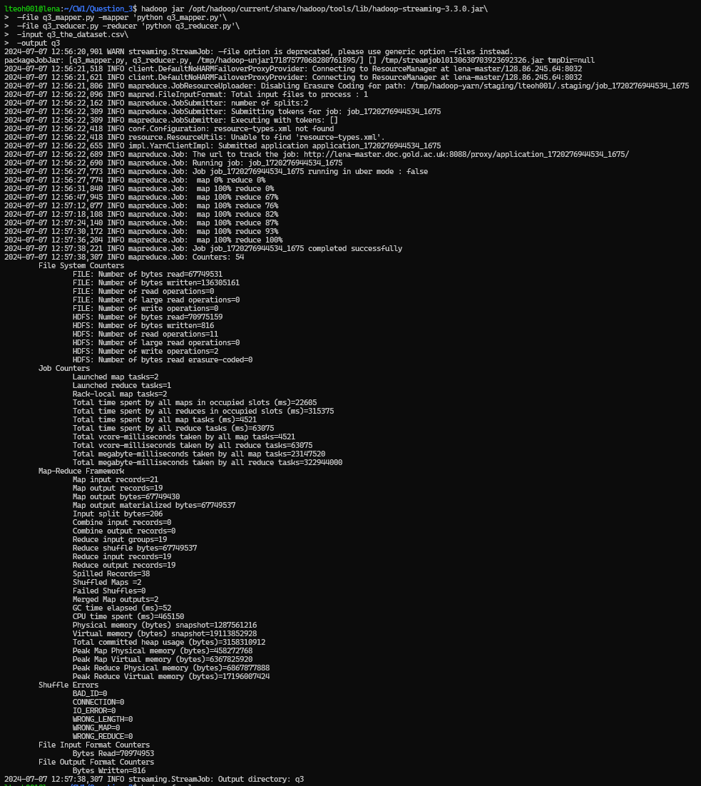

Then, we extract the output folder to our local file, and then reading the file in the output folder. Using the following commands:

hadoop fs -get q3
cd q3
cat part-0000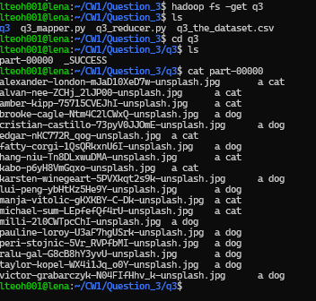

Based on the output, the model successfully classified the base-64 encoded image data into either "a dog" or "a cat" categories.

Back to Projects

Question 1 - Find the descriptive statistics for temperature of each day of a given month for the year 2007
Question 2 – Cluster Analysis using Apache Mahout
Question 3 - Use a classifier to distinguish between cats and dogs

Big Data Analysis - Using Hadoop for MapReduce, Cluster Analysis, and Image Classification

Table of Contents