Abstract
In this project, we compared a dataset from Romania with our own collected dataset from Malaysia. We explored how different factors like age, income, and education affect a person's financial literacy and financial well-being. We found that while things like education and income usually predict financial skills, our dataset showed some different and interesting behaviors. For example, we noticed that people with high income and high financial literacy in our group actually prefer 'mental tracking' instead of keeping strict records. We also found that even though our group had higher financial literacy scores, it didn't necessarily mean they had higher financial well-being scores compared to the Romanian group. We also observed that the financial well-being for our dataset didn't hit the 'universal security' levels that were seen in the Romanian dataset.
There is also a part 2 of this project, where we use the same romanian and self-surveyed dataset, along with a Ghanaians dataset, to also explore the relationship of sociodemographic and financial factors, in the participation of Higher Risk Financial Vehicle such as sport-betting, cryptocurrency, derivatives, forex, etc.
Research Topic
Topic of Investigation
Financial literacy has been a popular topic to explore, which can be seen in the number of publications and researches increasing year over year, as shown in this bibliographic analysis by Goyal and Kumar (2021). The aim of the research is to explore the relationship of between sociodemographic attributes and financial literacy and their effect on financial well-being and the avoidance of higher-risk financial vehicle (HRFV). In this study, a questionnaire survey will be conducted, as existing literature review have demonstrated the positive impact of financial literacy on financial well-being, as discussed in later sections. As for the aspect of avoiding risk financial, this will be the additional contribution to the study of financial literacy and also to understand if financial literacy makes an individual avoid higher-risk financial vehicles (HRFV) or encourage them to utilize it due to their better understanding of associated risks and financial management, such as the study by Ofosu and Kotey (2019).
This project is inspired by Nițoi et al. (2022) as the questionnaire from this study will be adopted, but focuses on target demographic of university students and working adults of Malaysians residing in Kuala Lumpur. The result of the project by Nițoi et al. (2022) will be used as data source for comparison against the outcome of this project. Additional questions to the questionnaire will be added to further explore the avoidance of HRFV, and will be compared to other existing studies such as the study by Ofosu and Kotey, (2019).
Background Research
Sociodemographic Attributes, Financial Literacy and Financial Well-Being
The findings in several studies, such as Zulfiqar and Bilal (2016), Zhang and Chatterjee (2023), Akhter and Sangmi (2016), have demonstrated a positive relationship between financial literacy and financial well-being. This is because financial literacy equips individuals with the skills to effectively plan and manage their finances, which reduces stress and anxiety that could be caused by unforeseen circumstances. These findings also emphasize the importance of policymakers, regulators, governments and educators taking proactive measures to improve and elevate financial literacy for everyone through educational program. As emphasized by Zhang and Chatterjee (2023), “it is never too late to educate individuals on financial literacy”.
This project will utilize a dataset (secondary data) from a study conducted in Romania, Nițoi et al. (2022). The study highlighted that 92% of the 1391 respondents in the questionnaire survey were financially illiterate. Results also indicated that only 15% felt financially secured, 35% had a moderately stable financial situation, 38% struggled to meet their financial needs, and the remaining 13% experienced significant financial insecurity. Income levels, age and education were identified as influential factors in determining financial well-being, while gender and residential status exhibited no significant impact. Furthermore, the study also noted that individuals with higher financial literacy, have above-average financial well-being.
Numerous studies have been conducted in Malaysia, in a variety of areas of financial literacy. Despite their limited citation, they offer valuable insights in a local perspective. For instance, in a study conducted by Kah et al. (2021), it was identified that sociodemographic attributes, including income, age and education level, along with financial literacy, played significant roles in the engagement of financial planning. This engagement in turn, results in achieving good financial well-being. Similarly, Ali et al. (2015) concluded that financial literacy was a crucial determinant for basic money management and financial planning, which are essential steps toward financial well-being. Notably, over 60% of the sampled Malaysian demonstrated moderately high levels of financial literacy. Furthermore, a study by Rahman et al. (2021) examined the financial well-being, financial stress, and financial literacy as variables. The results indicated that all three variables were statistically significant. Therefore, this project will explore into the relationship between sociodemographic attributes, financial literacy and financial well-being.
Operational Definitions
Financial Literacy
Nițoi et al., (2022) has adopted standardized approach for measuring financial literacy from a widely cited study by Lusardi and Mitchell, (2009) , where they have established a set of basic and advanced questions to assess an individuals’ financial literacy. This project will be using the same sets of questions and scoring to ensure comparability with the dataset from Nițoi et al., (2022).
Finacnial Well-Being
Nițoi et al., (2022) utilized the Consumer Financial Protection Bureau (CFPB)’s financial well-being questionnaire and scoring method to measure financial well-being. This widely accepted approach will be applied in this project as to ensure comparability with the dataset from Nițoi et al., (2022).
Research Objectives
- To understand the influence of sociodemographic attributes to financial literacy and financial well-being.
- To understand the relationship between financial literacy and financial well-being
Research Questions
- What are sociodemographic conditions that affect the financial literacy and financial well-being of an individual?
- Does possessing financial literacy lead to financial well-being?
Data Collection & Survey Design
Population and Sample
Based on data on Statista (2023), in the year 2020, there are around 500,000 students in university, and in year 2022, there were approximately 15 million that working adults (age range from 15 to 64). Because the population size is so large, and there is no data available to further narrow the scope to only university student and early working adults. Based on the calculation for ideal sample size, if at confidence level of 95% with margin of error of 5% and population of 50%, the sample size would be 385. Because the questionnaire survey that was made and the short time frame of this project, even at the margin of error of 10%, the sample size required is still 97. The goal for this project, is to get 97 to 385 responses.
In the end, the survey was able to reach about 144 response. We used Jisc Online Surveys, as it was required for the project. We have also employed word of mouth or similarly, snowball sampling. This was the easiest way, given the resource and time constraint for the given project. This method of data collection also has its downsides, such as having bias to the data. This is because, people around us are highly likely to have some form of similarity in characteristics, financial status and demographic traits with us. There is also a risk of data inaccuracy as participants might not take the survey as seriously. For our case, the demographic was supposed to be targeted to younger adults from 18 to 35 years old. But because of this method of collecting data, we ended up having a wide range of ages in the survey, which we will explore in the later sections.
The survey was available for participants for the month of September. We also gave the option for survey participants to claim an optional RM3 / £0.50 / US$0.63. Additionally, the response rate for the survey is 48%, about half of the participants completed the survey.
External Data Source
The project will be using a dataset from a study from Romania Nițoi et al. (2022), where a survey was conducted in regards to financial literacy and financial well-being. It was the only few full datasets which included the questionnaire and the data for a direct comparison.
We will be using an external dataset from the Romanian study, , which can be downloaded in the link of their paper, it contains all the relevant links to the paper, and for the dataset.
Another set of paper that we will be making comparison to is the Ghanaian study, Ofosu and Kotey, (2019). Note that a direct comparison between Ghana and Malaysia may not be entirely equal due to their differing financial situations. For instance, in 2021, Ghana’s GDP stood at US$77 billion while Malaysia’s GDP reached nearly US$373 billion, according to data from the World Bank, (2023). Although GDP alone does not fully reflect a country’s financial situation, it is often used as a quick indicator.
Key Findings
The key findings are:
Does High Financial Literacy mean High Financial Well-Being?
We found that our dataset had higher average financial literacy scores (peaking at 4 out of 8) compared to the Romanian dataset (peaking at 2 out of 8). However, having a higher score did not mean having better financial well-being. In fact, we saw that financial well-being scores for our dataset were capped at around 57.5, while the Romanian dataset had scores going above 70, reaching 'universal security' levels. Ironically, we also found a weak negative correlation (-0.12) between financial literacy and financial well-being in our dataset.
Do High Earners Keep Strict Records?
In the Romanian study, we saw that as people earn more and get older, they tend to keep better records of their money. But for our dataset, we found something different. We observed that those with high financial literacy actually do less strict recording and prefer 'Mental Tracking'. This suggests that they might feel confident enough to just estimate their finances mentally instead of keeping detailed records.
Who do we listen to for advice?
We found that the participants in our dataset, who are mostly urban Malaysians, rely a lot more on "Social Media" and "Advice From Family" for financial advice. This is different from the Romanian dataset, where they favor "Mass Media" (TV and Radio) and "Personal Experience". We also noted that the individuals with high financial well-being in our group relied less on professional financial advisors. This challenges the idea that once you have more money, you would hire a professional to manage it.
Does Gender affect Financial Outcomes?
For the Romanian dataset, we saw that financial well-being was quite equal between genders. However, in our dataset, we observed a difference. The group with "High Financial Well-Being" (those scoring 1 standard deviation above the mean) was mostly Male (about 75%), even though females had similar financial literacy scores in the middle ranges. This suggests there might be other factors affecting well-being outside of just financial knowledge.
Conclusion
So, to answer our initial research questions:
-
What are sociodemographic conditions that affect the financial literacy and financial well-being of an individual?
We found that education and income are generally good predictors for financial literacy, similar to what the Romanian study found. However, for financial well-being in our Malaysian context, being Male and having a higher income seemed to be the strongest traits for the "high well-being" group. Surprisingly, we also found that high income and education sometimes led to less strict financial recording, with people relying more on mental tracking.
-
Does possessing financial literacy lead to financial well-being?
In our study, the answer is: not necessarily. While participants in our dataset had higher financial literacy scores on average than the participants in the romanian dataset, this didn't translate to higher financial well-being scores. In fact, we found a weak negative link between the two. This suggests that just knowing about money isn't enough to guarantee feeling financially secure, especially for the younger urban demographic we surveyed.
Limitation of Research
Causaction and Correlation
The findings in this project are mainly correlation and relationship between factors and/or characteristics of the dataset and survey participants. We cannot fully conclude a direct causation in the findings. For example, it might be because of having higher financial literacy that causes one to have higher income due to having financial knowledge on how to manage money, But it also can be argued that because one has achieved a higher income, they will have increased financial literacy as it is needed to extend and further understand the management of money.
Sample Limitations
For our dataset, we were only able to achieve 144 survey responses and they are mainly based in Kuala Lumpur, one of the city area of Malaysia, and majority of them are young adults. Hence, it will not be a good representation of whole country of Malaysia. Additionally, because we employed word of mouth and snowball sampling method, we were able to extend the target audience to those that are above 35. However, they were not sufficient to build a good representation of these age group, which affects the findings later on, where trend and patterns might not be identifiable.
Data Pre-processing and Exploratory Analysis
Age Distribution
Because the survey was designed to collect discrete individual ages, rather than in range of age like (18 - 30, 31 - 40, etc), so that we can fine tune the data afterwards. We initially aim to collect data from survey participants aged between 18 to somewhere late 30s. Hence, during the survey design process, we decided to cap the age at 60, and allowed those above 60 to select the option ">60", if there were any. To ensure we had no input error/mistakes by the participates, we used drop down list from 18 to 60, and ">60".
Actual Distribution
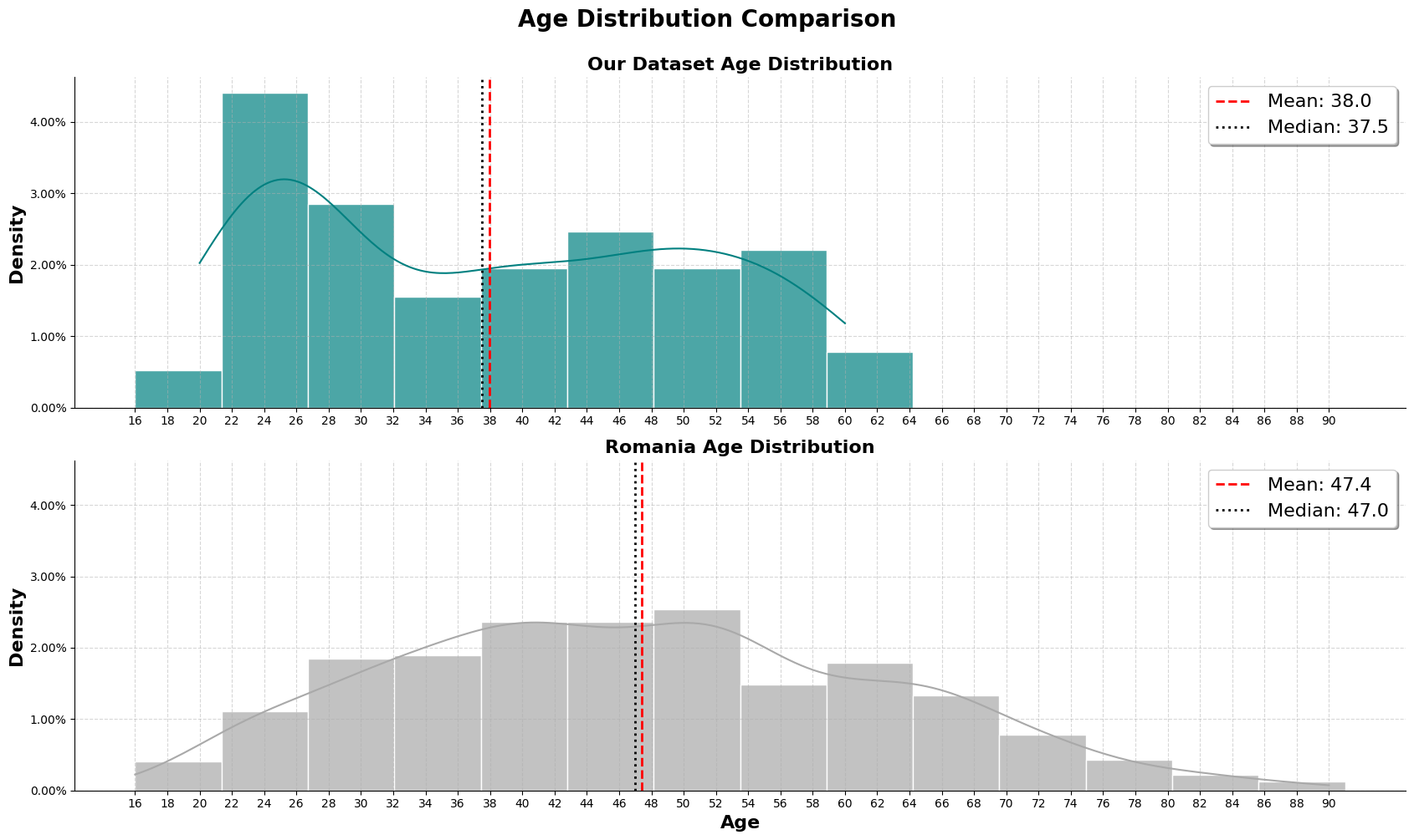
As shown in the graph, our dataset has a limitation where an individual might be older than 60, but it cannot be accurately shown in the graph. Our dataset heavily skewed towards 18 - 35, even with the limitation mentioned.
For the romanian dataset, we can observe that there is a good general spread of population throught the age range, peaking around the ages 40 - 60.
Treating 'above 60' as a group
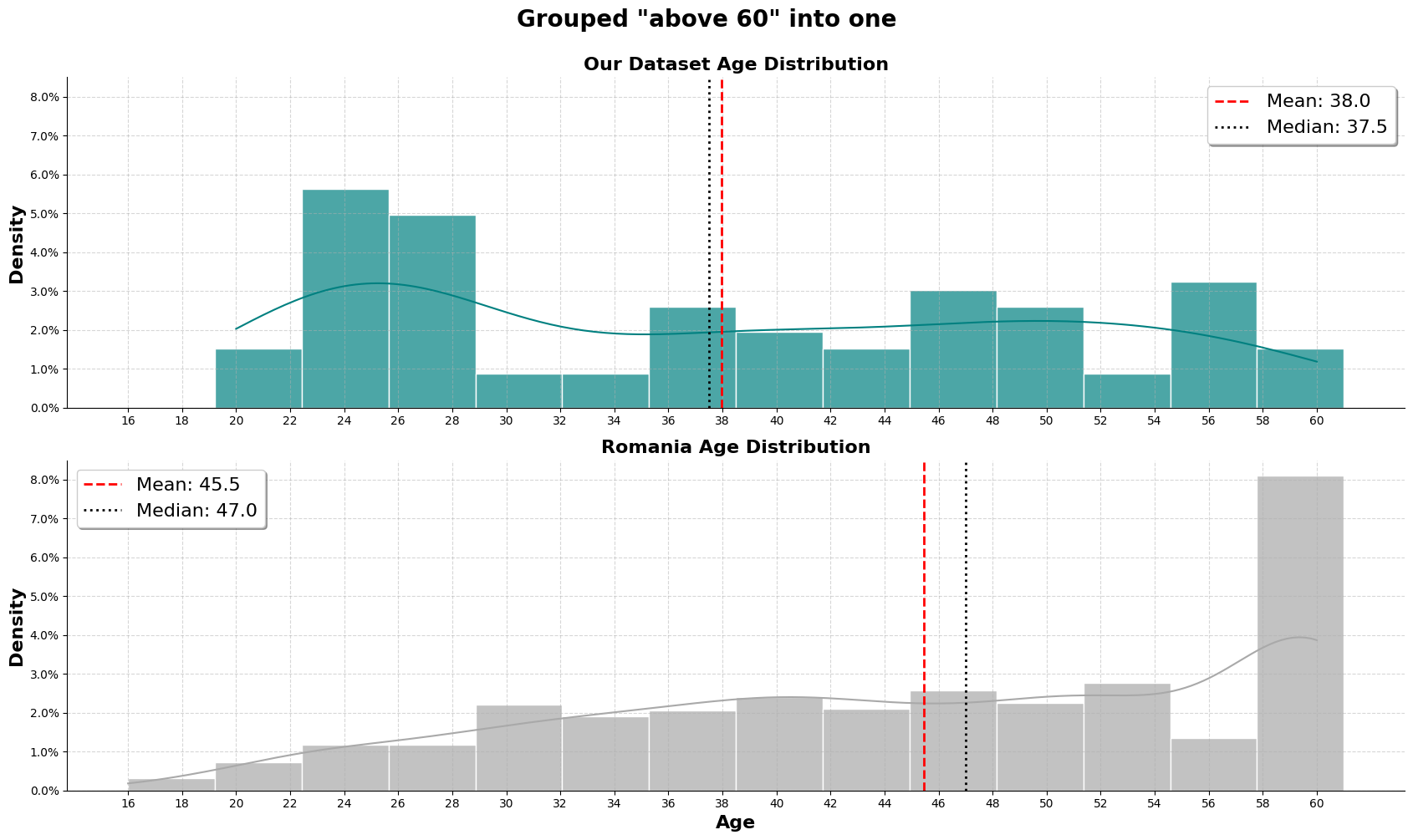
To apply the same standards between both dataset, we will treat those that are above 60, as one group. As shown in the graph, the romanian dataset will then have a heavy skew to the right, with over 8% of the population in the '>60' category.
Split into groups of 4, 12 years apart
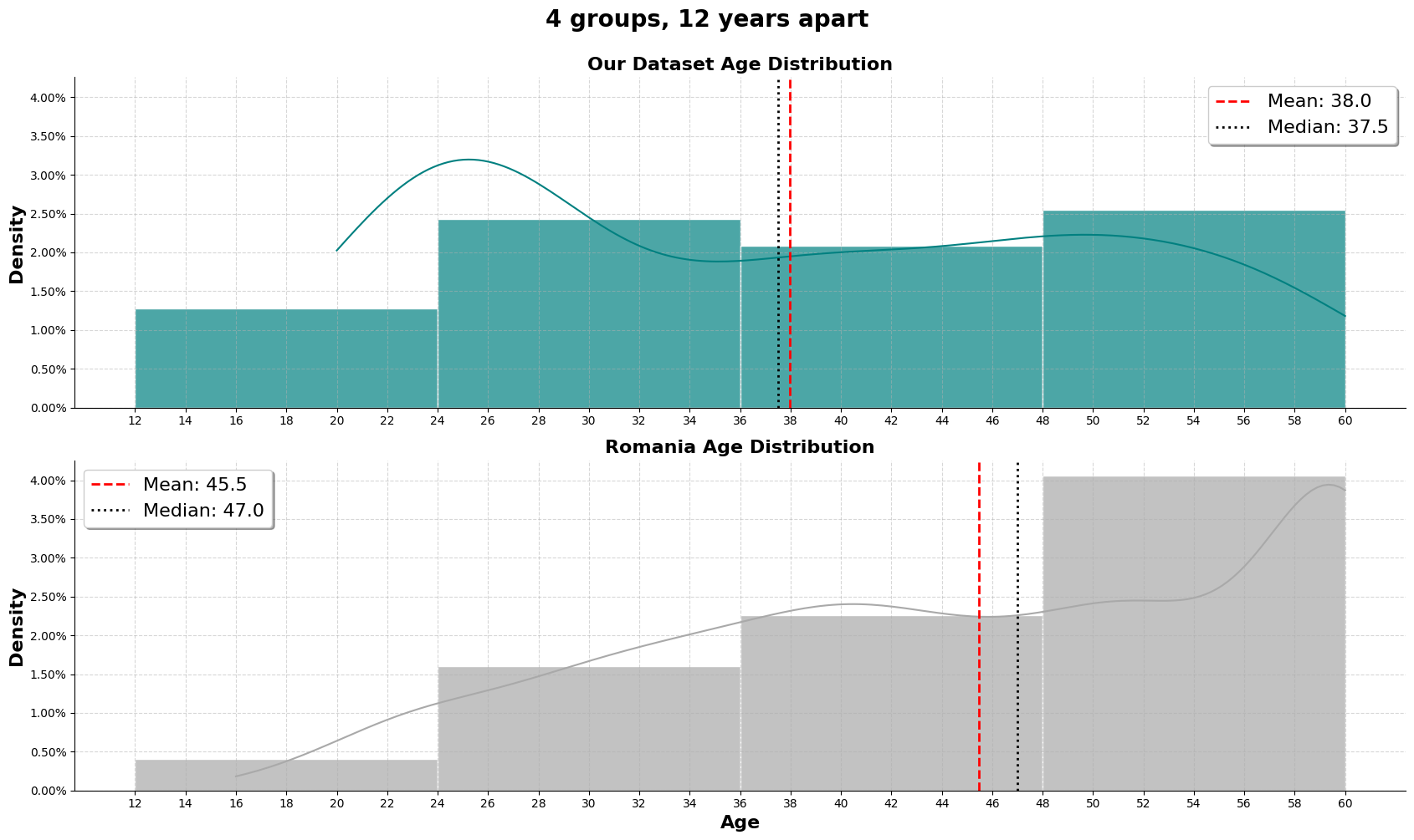
Then, proceeded to group them into 4 groups, 12 years apart. For our dataaset, the group seem to relatively equal for the last 3 groups, while for the romanian dataset, the split has made each ascending group to have more population. We are aware that the age bin of 12 - 24, even though there is no data indicating age of 16 and below, we decided to stick with it because during trial and error, the starting age of 12 and then continuously jumping 12 years for each group seem fitting.
def create_age_distribution_chart(our_dataset, romania_dataset, min_age, max_age, bin, suptitle):

    # Initialize figure
    fig, (ax1, ax2) = plt.subplots(2, 1, figsize=(17, 10), facecolor='white', sharey=True)

    # Setting values for loop
    datasets = [
        ('Our Dataset', our_dataset, 'teal', ax1),
        ('Romania', romania_dataset, 'darkgray', ax2)
    ]

    # Loop through the values set
    for country, df, color, ax in datasets:

        # Get age column
        age_col = 'SD3' if country == 'Romania' else [c for c in df.columns if 'age' in c.lower()][0]
        data = df[age_col]

        # Plot Histogram + KDE
        sns.histplot(data, bins=bin, kde=True, color=color, alpha=0.7, ax=ax, stat="density",
                     edgecolor='white', linewidth=1)

        # Set mean and median
        mean_val = data.mean()
        median_val = data.median()
        ax.axvline(mean_val, color='red', linestyle='--', linewidth=2, label=f'Mean: {mean_val:.1f}')
        ax.axvline(median_val, color='black', linestyle=':', linewidth=2, label=f'Median: {median_val:.1f}')

        # Styling
        ax.set_title(f'{country} Age Distribution', fontsize=16, fontweight='bold')
        if ax == ax2:
            ax.set_xlabel('Age', fontsize=16, fontweight='bold')
        else:
            ax.set_xlabel('')

        ax.set_ylabel('Density', fontsize=16, fontweight='bold')
        ax.set_xticks(range(min_age,max_age,2))

        ax.legend(frameon=True, fontsize=16, shadow=True)
        ax.grid(axis='x', alpha=0.5, linestyle='--')
        ax.grid(axis='y', alpha=0.5, linestyle='--')
        ax.spines['top'].set_visible(False)
        ax.spines['right'].set_visible(False)

    fig.suptitle(suptitle,
                 fontsize=20, fontweight='bold', y=1)

    formatter = mtick.PercentFormatter(xmax=1.0)
    ax.yaxis.set_major_formatter(formatter)

    plt.tight_layout()
    plt.show()


# Generate Plots
# ================

# Age Distribution Comparison
create_age_distribution_chart(our_dataset, romanian_dataset, 16, 91, np.linspace(16,91,15),
                              'Age Distribution Comparison')

# Replacing anything above 60, into 60
romanian_dataset['SD3'] = romanian_dataset['SD3'].where(
    romanian_dataset['SD3'] <= 60,  60
)

# Grouping 'above 60' as 60
create_age_distribution_chart(our_dataset, romanian_dataset, 16, 61, np.linspace(16,61,15),
                              'Grouped "above 60" into one')

# Splitting into groups of 4, 12 years apart
create_age_distribution_chart(our_dataset, romanian_dataset, 12, 61, np.histogram_bin_edges([12,24,36,48,60],4),
                              '4 groups, 12 years apart')
Gender Distribution
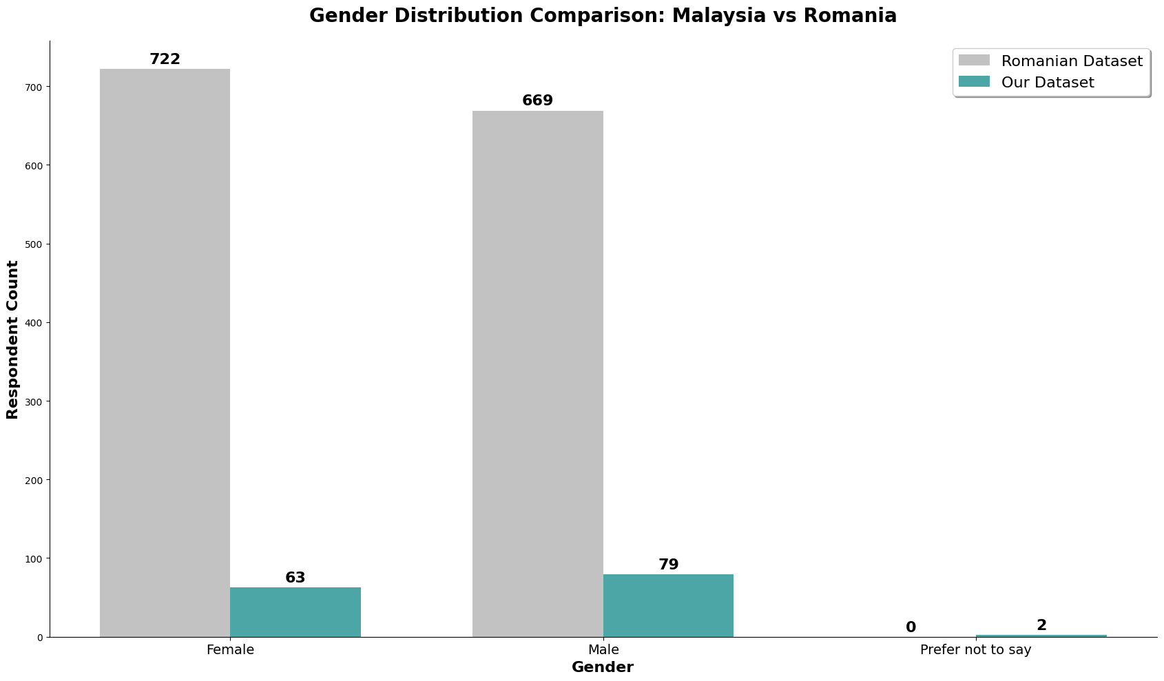
The chart above is the gender count for both datasets.
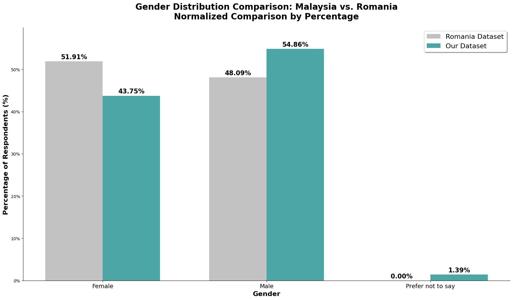
The chart above is the gender count normalized. We can observe that the romanian dataset has almost a perfect 50/50, almost 4% more females. On the other hand, our dataset has about 11% more males, in which we should take note in our analysis later.
# Data Preparation
# ================
# Set labels
genders = ["Female", "Male", "Prefer not to say"]

# Get the count of the unique values of both datasets
romanian_dataset_gender_count = getCount(romanian_dataset['SD2'])
our_dataset_gender_count = getCount(our_dataset[getOurString('gender', our_columns)])

# Adding 'Prefer not to say' to Romania
romanian_dataset_gender_count["Prefer not to say"] = 0

# Sorting them
romanian_dataset_gender_count = dict(sorted(romanian_dataset_gender_count.items()))
our_dataset_gender_count = dict(sorted(our_dataset_gender_count.items()))

# Store and sort gender ratio
our_dataset_gender_ratio = our_dataset_gender_count.copy()
for key in our_dataset_gender_ratio:
    our_dataset_gender_ratio[key] /= our_total_respondent
our_dataset_gender_ratio = dict(sorted(our_dataset_gender_ratio.items()))

romanian_dataset_gender_ratio = romanian_dataset_gender_count.copy()
for key in romanian_dataset_gender_ratio:
    romanian_dataset_gender_ratio[key] /= romanian_total_respondent
romanian_dataset_gender_ratio = dict(sorted(romanian_dataset_gender_ratio.items()))

gender_ratio_datasets = [romanian_dataset_gender_ratio, our_dataset_gender_ratio]

# Count Chart
# ==============
# Initialize the plots using Object-Oriented API
fig, ax = plt.subplots(figsize=(17, 10))

# Set x values and
x = np.arange(3)
width = 0.35

#  Plot both datasets on same axes with appropriate offsets
bar1 = ax.bar(x - width / 2, romanian_dataset_gender_count.values(), width,
              label='Romanian Dataset', color='darkgray', alpha=0.7)
ax.bar_label(bar1, padding=3, fontsize=16, fontweight="bold")

bar2 = ax.bar(x + width / 2, our_dataset_gender_count.values(), width,
              label='Our Dataset', color='teal', alpha=0.7)
ax.bar_label(bar2, padding=3, fontsize=16, fontweight="bold")


# Styling
ax.set_title('Gender Distribution Comparison: Malaysia vs Romania',
             fontsize=20, fontweight='bold', pad=20)
ax.set_xlabel('Gender', fontsize=16, fontweight="bold")
ax.set_ylabel('Respondent Count', fontsize=16, fontweight="bold")

ax.legend(frameon=True, shadow=True, fontsize=16)

ax.set_xticks(x)
ax.set_xticklabels(genders, fontsize=14)

ax.spines['top'].set_visible(False)
ax.spines['right'].set_visible(False)

plt.tight_layout()
plt.show()

# Percentage Chart
# ================
# Create Plot
fig, ax = plt.subplots(figsize=(17,10))

# Set x values and width
x = np.arange(3)
width = 0.35

# Plot both datasets on same axes with appropriate offsets
bar1 = ax.bar(x - width/2, gender_ratio_datasets[0].values(), width,  label="Romania Dataset", color="darkgray", alpha=0.7)
bar2 = ax.bar(x + width/2, gender_ratio_datasets[1].values(), width, label="Our Dataset", color="teal", alpha=0.7)

for bar in [bar1, bar2]:
    ax.bar_label(bar, fmt='{:.2%}', fontsize=15, fontweight='bold', padding=3)

# Styling
ax.set_ylabel('Percentage of Respondents (%)', fontsize=16, fontweight='bold')
ax.set_xlabel('Gender', fontsize=16, fontweight='bold')

ax.set_title('Gender Distribution Comparison: Malaysia vs. Romania\nNormalized Comparison by Percentage',
                fontsize=20, fontweight='bold', pad=20)

ax.set_xticks(x)
ax.set_xticklabels(genders, fontsize=14)

ax.set_ylim(0, max(max(gender_ratio_datasets[0].values()), max(gender_ratio_datasets[1].values())) + 0.05)
ax.legend(shadow=True, frameon=True, fontsize=16)

ax.spines['right'].set_visible(False)
ax.spines['top'].set_visible(False)

formatter = mtick.PercentFormatter(xmax=1.0)
ax.yaxis.set_major_formatter(formatter)

plt.tight_layout()
plt.show()
Education Attainment
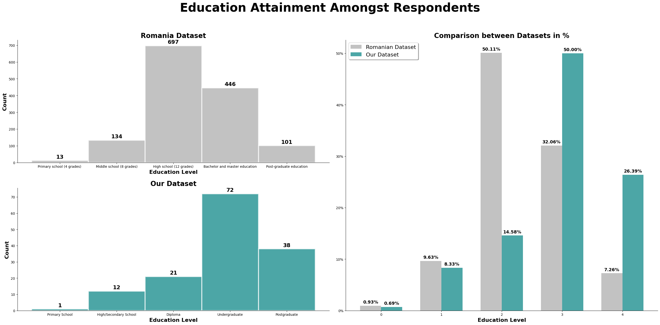
This chart above is a combined chart. It shows the number of respondent and the education level attained. The plot on the left shows the normalized value of both dataset, so we can compare to it directly.
However, we also need to take note that there are differences between the education level listed in both survey. The third level of education attaiment for the romanian dataset is 'High School (12 Grade)', which is equivalent to a college entrance exam, or Form 6 in Malaysia. However, taking up Form 6 level education in Malaysia is not a common education path, especially in Kuala Lumpur. Hence, we have made the changes to the survey question, changing 'High School (12 Grade)' to 'Diploma', making the 3rd level of education attainment not directly comparable, do refer the following link for more details on the changes made from the romanian study.
We can observe that for the romanian dataset, most of the respondents' highest education attainment is 'High School (12 Grade)'. For our dataset, it is an undergraduate degree. Both dataset has 50% of the respondents obtaining the respective common education attainment.
# Data Prepartion
# =================
# Store the column
romanian_dataset_education = romanian_dataset['SD4']

# Print the unique values
print('Unique Values (Romanian Dataset): ', list(set(romanian_dataset_education)))

# Assign a value to the unique values, according to the level of education
custom_dict_romania_education = {
    'Primary school (4 grades) ': 0,
    'Middle school (8 grades)': 1,
    'High school (12 grades)': 2,
    'Bachelor and master education': 3,
    'Post-graduate education': 4
}

# Sort the dataset according the custom dict above
romanian_dataset_education = romanian_dataset_education.sort_values(
    key=lambda x: x.map(custom_dict_romania_education))

# Get the count of all unique values
romanian_dataset_education_dict = getCount(romanian_dataset_education)

# Get the column string for educational attainment
our_dataset_education_string = [column for column in our_columns if 'educational' in column][0]

# Store the column
our_dataset_education = our_dataset[our_dataset_education_string]

# Print the unique values
print('Unique Values (Our Dataset): ', list(set(our_dataset_education)))

# Assign a value to the unique values, according to the level of education
custom_dict_our_education = {
    'Primary School':0,
    'High/Secondary School':1,
    'Diploma':2,
    'Undergraduate':3,
    'Postgraduate': 4
}

# Sort the dataset according to the custom dict above
our_dataset_education = our_dataset_education.sort_values(key=lambda x: x.map(custom_dict_our_education))

# Get the count of all unique values
our_dataset_education_dict = getCount(our_dataset_education)

# Store the educational attainment
romanian_dataset['Educational Attainment'] = romanian_dataset['SD4'].map(custom_dict_romania_education)
our_dataset['Educational Attainment'] = our_dataset[our_dataset_education_string].map(custom_dict_our_education)

# Create percentage/ratio dataset
our_dataset_education_dict_ratio = our_dataset_education_dict.copy()
romanian_dataset_education_dict_ratio = romanian_dataset_education_dict.copy()

for key in our_dataset_education_dict_ratio:
    our_dataset_education_dict_ratio[key] /= our_total_respondent

for key in romanian_dataset_education_dict_ratio:
    romanian_dataset_education_dict_ratio[key] /= romanian_total_respondent

# Plot Figure
# ============
# Getting Labels
our_education_labels = list(our_dataset_education_dict.keys())
romanian_education_labels = list(romanian_dataset_education_dict.keys())

# Set figure
fig = plt.figure(layout='constrained', figsize=(27,12))
gs = GridSpec(2, 2, figure=fig) # Set two 2 x 2 grid
ax1 = fig.add_subplot(gs[0, 0]) # takes grid position 0,0 - top left
ax2 = fig.add_subplot(gs[1, 0]) # takes grid position 1,0 - bottom left
ax3 = fig.add_subplot(gs[:, 1]) # takes grid position :,0 - full right

fig.suptitle("Education Attainment Amongst Respondents", fontsize=35, fontweight='bold', y=1.1)

# Set x values and width
x = np.arange(5)
width = 0.35

# Set values to loop
datasets = [
    ('Romania Dataset', romanian_dataset_education_dict.values(), romanian_education_labels , 'darkgray', ax1),
    ('Our Dataset',our_dataset_education_dict.values(), our_education_labels, 'teal', ax2)
]

# First Column
# ==============
# Looping through values
for title, dataset, labels, color, ax in datasets:

    # Set bar
    bar = ax.bar(x, dataset, width=1, label=title, color=color, alpha=0.7, edgecolor='white', linewidth=3)

    # Styling
    ax.set_title(title, fontweight='bold', fontsize=20)
    ax.set_ylabel('Count', fontweight='bold', fontsize='16')
    ax.set_xlabel('Education Level', fontweight='bold', fontsize='16')

    ax.bar_label(bar, padding=3, fontsize=16, fontweight='bold')
    ax.set_xticks(x)
    ax.set_xticklabels(labels)

    ax.spines[['top', 'right']].set_visible(False)

# Second Column
# ==============
# Set bar
bar1 = ax3.bar(x - width/2, romanian_dataset_education_dict_ratio.values(), width, label = 'Romanian Dataset', color='darkgray', alpha=0.7)
bar2 = ax3.bar(x + width/2, our_dataset_education_dict_ratio.values(), width, label='Our Dataset', color='teal', alpha=0.7)

# Set bar labels
for bar in [bar1, bar2]:
    ax3.bar_label(bar, fmt='{:.2%}', fontsize=13, fontweight='bold', padding=4)

# Styling
ax3.spines[['top', 'right']].set_visible(False)
ax3.legend(shadow=True, fontsize=16, loc='upper left')
ax3.set_xlabel('Education Level', fontweight='bold', fontsize='16')
ax3.set_title('Comparison between Datasets in %', fontweight='bold', fontsize=20)
formatter = mtick.PercentFormatter(xmax=1.0)
ax3.yaxis.set_major_formatter(formatter)

plt.show()
Income Distribution
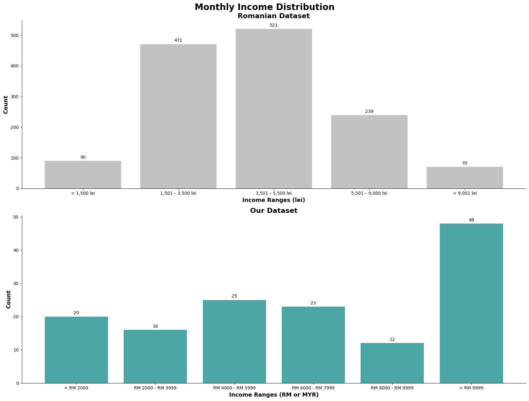
One thing to note is that, based on International Monetary Fund, for the Romanian Stats, and for the Malaysian stat. As of October 2023, we can see that Malaysia's GDP is US$430.90 billion, and the GDP per capita is US$13.03 thousands while for Romania, their GDP is US$350.41 billion and the GDP per capita is US$18.41 thousands. GDP and GDP per capita is not the ultimate financial indicator, but it is usually used as a quick overview, based on this finding, we can see that both economies have similar, but Romania has better GDP per capita as they have a population of 19 million people while Malaysia has 33 million. Additionally, 1 Romanian Leu is equivalent to 1.02 Malaysia Ringgit, which further shows the similarity in financial performance of the two countries.
Based on the chart above, we can observe that they are many survey participants in our dataset making above the given income range set in the survey question. We will further explore income again later, like the sociodemographic make up for those who earned above RM9999. As mentioned in earlier section, there is a bias of the target audience specifically being in the area of Kuala Lumpur.
For the romanian dataset, we can see that the graph resemble a normal distribution. Meanwhile, for our dataset, about 33% of are in the '>RM9999', with an almost equal spread around the other price ranges.
# Data Preparation
# =================
romanian_dataset_income = romanian_dataset['SD7']
our_dataset_income_string = [column for column in our_columns if ' income' in column][0]
our_dataset_income = our_dataset[our_dataset_income_string]

# Print to check values - to create custom dict
print('Unique Values (Romanian Dataset):', list(set(romanian_dataset_income)))
print('Unique Values (Our Dataset): ', list(set(our_dataset_income)))

# Custom dict for sorting
custom_dict_romania_income = {
    '< 1,500 lei': 0,
    '1,501 – 3,500 lei': 1,
    '3,501 – 5,500 lei': 2,
    '5,501 – 9,000 lei': 3,
    '> 9,001 lei': 4
}
custom_dict_our_income = {
    '< RM 2000':0,
    'RM 2000 - RM 3999':1,
    'RM 4000 - RM 5999':2,
    'RM 6000 - RM 7999':3,
    'RM 8000 - RM 9999':4,
    '> RM 9999':5,
}

# Sort the column based on the custom dict
romanian_dataset_income = romanian_dataset_income.sort_values(
    key=lambda x: x.map(custom_dict_romania_income)
)
our_dataset_income = our_dataset_income.sort_values(
    key=lambda x: x.map(custom_dict_our_income)
)

# Get the count values for each of the dataset
romanian_dataset_income_dict = getCount(romanian_dataset_income)
our_dataset_income_dict = getCount(our_dataset_income)

# Plot Figure
# =============
# Initialize figure
fig, (ax1, ax2) = plt.subplots(2, 1, figsize=(17, 13))

fig.suptitle('Monthly Income Distribution',
             fontweight="bold", size=20)

# Set values for loop
datasets = [
    (romanian_dataset_income_dict, 'darkgray', 'lei', 'Romanian Dataset', ax1),
    (our_dataset_income_dict, 'teal', 'RM or MYR', 'Our Dataset', ax2)
]

# Loop values
for dataset, color, currency, title, ax in datasets:

    # Set bar
    bar = ax.bar(dataset.keys(), dataset.values(), color=color, alpha=0.7)

    # Styling
    ax.bar_label(bar, padding=3)
    ax.set_xlabel(f'Income Ranges ({currency})', fontsize=13, fontweight='bold')
    ax.set_ylabel('Count', fontsize=13, fontweight='bold')
    ax.set_title(title, fontsize=16, fontweight='bold')
    ax.spines[['top', 'right']].set_visible(False)

plt.tight_layout()
plt.show()
Financial Behaviour
In the surveys that were conducted on our own and the Romanian study, the questions in the Financial Behaviour section were not easily coverted into quantitative or relative value that can be used to compare, except for the act of keep financial records. Hence, we will be using 'Financial Recording' question, and converting into a quantitative value. The list of questions relevant to Financial Behaviour, can be referred in the link.
Financial Recording
This is the question in the survey:
- Yes, we keep records of all revenues and all expenses.
- Yes, we keep records, but not all revenues and expenses are recorded.
- No, we don’t keep records, but we know how much money we earn and spend during a month.
- No, we don’t keep records, and we don’t know how much money we earn and spend during a month.
For the sake of simplifying the graph, we will convert the answers 1 - 4 shown above, to 'Full Recording', 'Partial Recording', 'Mental Recording' and 'No Recording'.
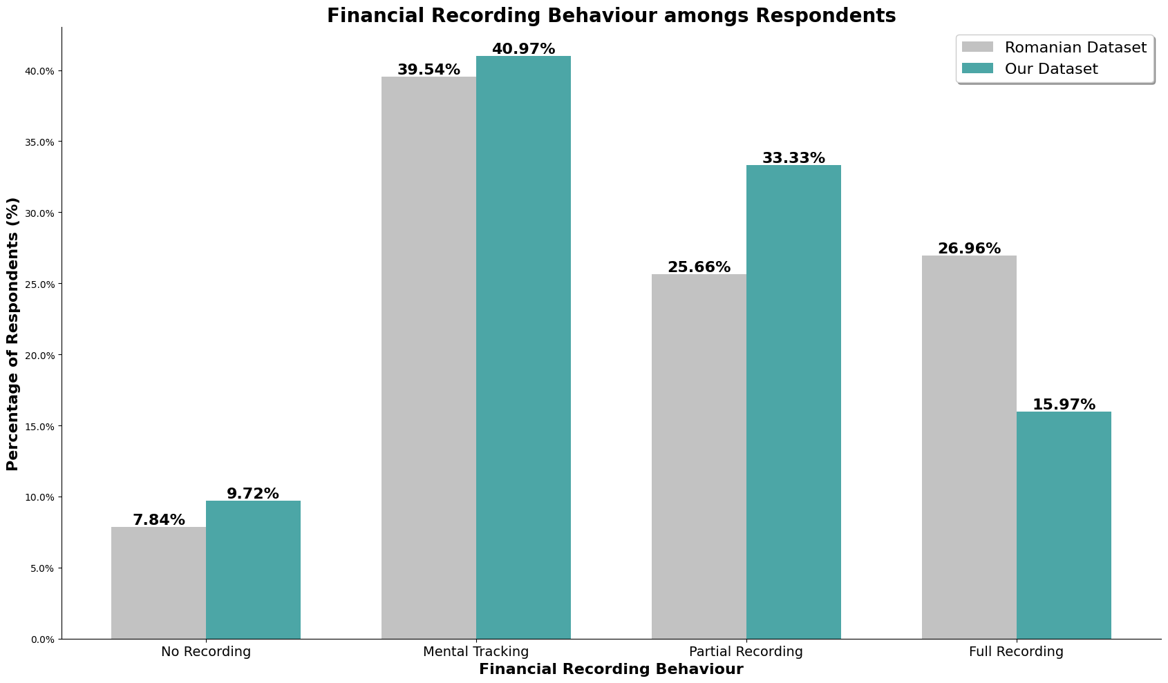
The above chart is the normalized value for both the dataset, so we can directly compare it. For the romanian dataset, there is about a quarter of its population that does full recording, and our dataset, there is only about 15% that does full recording. Majority population for both our and the romanian dataset only does mental tracking, where they do not keep track but understands their incomes and spending. Our dataset also has higher number of survey participants (almost 10%) who does not track at all when compared to the romanian dataset, almost 8%.
Our dataset may consist of higher number of high-earners, but we still observe our dataset having more participants that do not track their incomes and expenses, and lesser number of participants performing full recording. It could also be because our dataset is skewed to a younger audience, which is still picking up and honing their financial management skills, or it could be because high-earners is able to afford not full tracking to not tracking their income and expenses when they have understand the financial structure and habits that has been established.
# Data Preparation
# ==================

# Get our column
our_finance_record_string = getOurString(
    'Do you or other person in your household keep a record of income and expenses on a monthly basis?',
    our_columns)

our_dataset_finance_record = our_dataset.filter(
    items=[
        our_age_string,
        our_finance_record_string
    ])

# Get romanian column
romanian_dataset_finance_record = romanian_dataset.filter(items=['SD3','I1'])

# Print unique values for custom dict
print(romanian_dataset_finance_record['I1'].unique())
print(our_dataset_finance_record[our_finance_record_string].unique())

# Create custom dict / value representation
custom_dict_our_financial_record = {
    'Yes, we keep records of all income and all expenses':0,
    'Yes, we keep records, but not all income and expenses are recorded':1,
    'No, we don’t keep records, but we know how much money was spent during a month':2,
    'No, we don’t keep records, and we don’t know how much money was spent during a month':3
}

custom_dict_romanian_financial_record = {
    'Yes, we keep records of all revenues and all expenses':0,
    'Yes, we keep records, but not all revenues and expenses are recorded':1,
    'No, we don’t keep records, but we know how much money we earn and spend during a month': 2,
    'No, we don’t keep records, and we don’t know how much money we earn and spend during a month':3
}

reverse_values = {0: 3, 1: 2, 2: 1, 3: 0}

romanian_dataset['Financial Recording'] = \
    romanian_dataset['I1'].map(custom_dict_romanian_financial_record)\
        .map(reverse_values)

our_dataset['Financial Recording'] = \
    our_dataset[our_finance_record_string].map(custom_dict_our_financial_record)\
        .map(reverse_values)

our_dataset_financial_recording_dict = our_dataset['Financial Recording']\
    .value_counts(normalize=True)\
    .sort_index().to_dict()

romanian_dataset_financial_recording_dict = romanian_dataset['Financial Recording']\
    .value_counts(normalize=True)\
    .sort_index().to_dict()

# Plot Figure
# ===========
# Create figure
fig, ax = plt.subplots(figsize=(17,10))

# Custom Label
financial_recording_label = ['No Recording', 'Mental Tracking', 'Partial Recording', 'Full Recording' ]

# Set x values and width
x = np.arange(4)
width = 0.35

# Plot both datasets on same axes with appropriate offsets
bar1 = ax.bar(x - width/2, romanian_dataset_financial_recording_dict.values(), width, label='Romanian Dataset',
              color='darkgray', alpha=0.7)
bar2 = ax.bar(x + width/2, our_dataset_financial_recording_dict.values(), width, label='Our Dataset',
              color='teal', alpha=0.7)

for bar in [bar1, bar2]:
    ax.bar_label(bar, fontsize='16', fontweight='bold', fmt='{:.2%}')

# Styling
ax.set_title('Financial Recording Behaviour amongs Respondents', fontsize='20', fontweight='bold')
ax.set_ylabel('Percentage of Respondents (%)', fontsize=16, fontweight='bold')
ax.set_xlabel('Financial Recording Behaviour', fontsize=16, fontweight='bold')
ax.set_xticks(x)
ax.set_xticklabels(financial_recording_label, fontsize=14)
ax.spines[['top', 'right']].set_visible(False)
ax.legend(shadow=True, fontsize='16')
formatter = mtick.PercentFormatter(xmax=1.0, decimals=None)
ax.yaxis.set_major_formatter(formatter)

plt.tight_layout()
plt.show()
Financial Literacy
Based on the Romanian study, financial literacy is calculate by the sum of all the correct answer, each having 1 point, and a maximum of 8. They have included the 'Big Three' and 'Big Five' question, referenced from Lusardi and Mitchell. This can be seen being utilized by Global Financial Literacy Excellence Center shown in the following link. The 'Big Three' and 'Big Five' Questions for Financial Literacy.. Also, by the Financial Industry Regulatory Authority (FINRA), as shown in the following link, financial knowlege quiz by FINRA.
So, we have to aggregate the scores from the survey and get the financial literacy score for each particpants. The list of questions in the survey can be referred here.
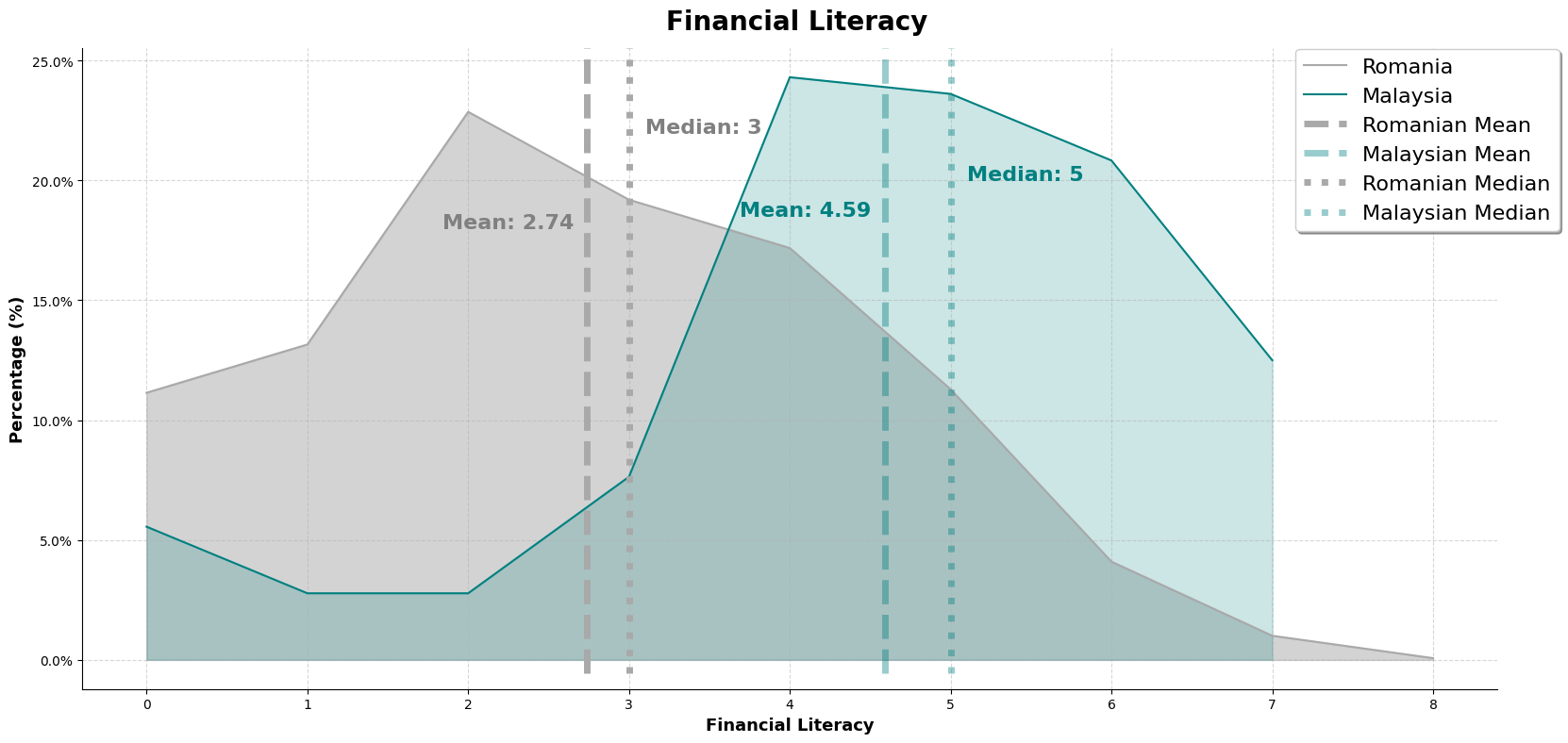
As shown by the result, there are a higher percentage of romanian participants scoring 2 while malaysian participants are scoring at 4. This is also evident by the mean and median line shown. But there are instances of romanian participants scoring above 6 while malaysian does not have any. We will further explore the relationship between financial literacy, financial well being and the sociodemographic and financial attitudes factors.
# Score Aggregation
# ==================

# Function to replace values in the column
def replace_values(col_no, answer, dataset, col_set):

    # Replacing correct answer with 1
    dataset[col_set[col_no]] = dataset[col_set[col_no]].replace(answer, 1)

    # Replacing wrong answer with 0
    dataset[col_set[col_no]] = np.where(
        dataset[col_set[col_no]] != 1, 0, dataset[col_set[col_no]]
    )

    return dataset

# To store the required columns -- For Romanian Dataset
romanian_financial_literacy_columns = []

# Base String
base_string = 'C'

# Loop from 1 to 8
for sub_string in range(1,9):
    romanian_financial_literacy_columns.append(
        base_string + str(sub_string)
    )

# To store the require columns -- For Our Dataset
our_financial_literacy_columns = [our_columns[x] for x in range(42,50)]


# Printing unique values for reference
for col in romanian_financial_literacy_columns:
    print(romanian_dataset[col].unique())

# Printing unique values for reference
for col in our_financial_literacy_columns:
    print(our_dataset[col].unique())


# Coverting answeres into values
# =====================================
romanian_financial_literacy = romanian_dataset[romanian_financial_literacy_columns]
our_financial_literacy = our_dataset[our_financial_literacy_columns]

# Probability
column_no = 0
romanian_financial_literacy = replace_values(
    column_no, '1 in 1,000,000', romanian_financial_literacy, romanian_financial_literacy_columns
)
our_financial_literacy = replace_values(
    column_no, '1 in 100000', our_financial_literacy, our_financial_literacy_columns
)

# Interest Rate
column_no = 1
romanian_financial_literacy = replace_values(
    column_no, 'More than LEI 150 ', romanian_financial_literacy, romanian_financial_literacy_columns
)
our_financial_literacy = replace_values(
    column_no, 'More than $150', our_financial_literacy, our_financial_literacy_columns
)

# Loan Repayment
column_no = 2
romanian_financial_literacy = replace_values(
    column_no, 'True', romanian_financial_literacy, romanian_financial_literacy_columns
)
print(our_financial_literacy[our_financial_literacy_columns[column_no]].unique())
our_financial_literacy = replace_values(
    column_no, 'True', our_financial_literacy, our_financial_literacy_columns
)

# Time value of money
column_no = 3
romanian_financial_literacy = replace_values(
    column_no, 'My friend', romanian_financial_literacy, romanian_financial_literacy_columns
)
our_financial_literacy = replace_values(
    column_no, 'My friend', our_financial_literacy, our_financial_literacy_columns
)

# Inflation
column_no = 4
romanian_financial_literacy = replace_values(
    column_no, 'The same', romanian_financial_literacy, romanian_financial_literacy_columns
)
our_financial_literacy = replace_values(
    column_no, 'The Same', our_financial_literacy, our_financial_literacy_columns
)

# Investment
column_no = 5
romanian_financial_literacy = replace_values(
    column_no, 'Multiple business of investments', romanian_financial_literacy, romanian_financial_literacy_columns
)
our_financial_literacy = replace_values(
    column_no, 'Multiple Business of Investment', our_financial_literacy, our_financial_literacy_columns
)

# Asset
column_no = 6
romanian_financial_literacy = replace_values(
    column_no, 'Stocks', romanian_financial_literacy, romanian_financial_literacy_columns
)
our_financial_literacy = replace_values(
    column_no, 'Stocks', our_financial_literacy, our_financial_literacy_columns
)

# Risk
column_no = 7
romanian_financial_literacy = replace_values(
    column_no, 'Stocks', romanian_financial_literacy, romanian_financial_literacy_columns
)
our_financial_literacy = replace_values(
    column_no, 'Stocks', our_financial_literacy, our_financial_literacy_columns
)

# Data Preparation
# ==================
# Getting the score
romanian_financial_literacy['Financial Literacy Score'] = \
    romanian_financial_literacy[romanian_financial_literacy_columns]\
        .sum(axis=1).astype(int)

our_financial_literacy['Financial Literacy Score'] = \
    our_financial_literacy[our_financial_literacy_columns]\
        .sum(axis=1).astype(int)

romanian_dataset['Financial Literacy Score'] = romanian_financial_literacy['Financial Literacy Score']
our_dataset['Financial Literacy Score'] = our_financial_literacy['Financial Literacy Score']

# Get unique values of the financial well being index, and sort them in ascending order
# The plot will get wonky if it is not in order
romanian_financial_literacy_x = \
    np.sort(romanian_financial_literacy['Financial Literacy Score'].unique())

our_financial_literacy_x = \
    np.sort(our_financial_literacy['Financial Literacy Score'].unique())

# Get the value count of each score, and then divide it by the size of each dataset
romanian_financial_literacy_y = \
    romanian_financial_literacy['Financial Literacy Score']\
    .value_counts().get(romanian_financial_literacy_x)\
    / len(romanian_financial_literacy)

our_financial_literacy_y = \
    our_financial_literacy['Financial Literacy Score']\
    .value_counts().get(our_financial_literacy_x)\
    /len(our_financial_literacy)

# Get the mean value for financial literacy score
romanian_financial_literacy_mean = romanian_financial_literacy['Financial Literacy Score'].mean()
our_financial_literacy_mean = our_financial_literacy['Financial Literacy Score'].mean()

# Get the median values for financial literacy score
romanian_financial_literacy_median = romanian_financial_literacy['Financial Literacy Score'].median()
our_financial_literacy_median = our_financial_literacy['Financial Literacy Score'].median()

# Get the standard deviation value for financial literacy score
romanian_financial_literacy_std = romanian_financial_literacy['Financial Literacy Score'].std()
our_financial_literacy_std = our_financial_literacy['Financial Literacy Score'].std()

# Initializing the figure
figure, ax = plt.subplots(figsize=(17,8))
figure.suptitle(
    'Financial Literacy',
    fontweight = 'bold',
    fontsize = 20
)

# Plot romania data
# =================
ax.plot(
    romanian_financial_literacy_x,
    romanian_financial_literacy_y,
    color = 'darkgray',
    label = 'Romania'
)

ax.fill_between(
    romanian_financial_literacy_x,
    romanian_financial_literacy_y,
    alpha = 0.5,
    color = 'darkgray'
)

# Plot our data
# ==============
ax.plot(
    our_financial_literacy_x,
    our_financial_literacy_y,
    color = 'teal',
    label = 'Malaysia'
)

ax.fill_between(
    our_financial_literacy_x,
    our_financial_literacy_y,
    alpha = 0.2,
    color = 'teal'
)

# Mean line and annotations
# ==========================
ax.axvline(
    romanian_financial_literacy_mean,
    0.025,
    ls = '--',
    color = 'darkgray',
    label = 'Romanian Mean',
    linewidth = 5
)

ax.annotate(
    f"Mean: {romanian_financial_literacy_mean:.3g}",
    xy=(romanian_financial_literacy_mean - 0.9 ,0.18),
    fontsize=16, fontweight='bold', color='grey')

ax.axvline(
    our_financial_literacy_mean,
    0.025,
    ls = '--',
    color = 'teal',
    label = 'Malaysian Mean',
    alpha = 0.4,
    linewidth = 5
)

ax.annotate(
    f"Mean: {our_financial_literacy_mean:.3g}",
    xy=(our_financial_literacy_mean - 0.9 ,0.185),
    fontsize=16, fontweight='bold', color='teal')


# Median Line and annotations
# =============================
ax.axvline(
    romanian_financial_literacy_median,
    0.025,
    ls = ':',
    color = 'darkgray',
    label = 'Romanian Median',
    linewidth = 5
)

ax.annotate(
    f"Median: {romanian_financial_literacy_median:.3g}",
    xy=(romanian_financial_literacy_median + 0.1 ,0.22),
    fontsize=16, fontweight='bold', color='grey')

ax.axvline(
    our_financial_literacy_median,
    0.025,
    ls = ':',
    color = 'teal',
    label = 'Malaysian Median',
    alpha = 0.4,
    linewidth = 5
)

ax.annotate(
    f"Median: {our_financial_literacy_median:.3g}",
    xy=(our_financial_literacy_median + 0.1 ,0.20),
    fontsize=16, fontweight='bold', color='teal')

# Styling
ax.set_ylabel('Percentage (%)', fontsize=13, fontweight='bold')
ax.set_xlabel('Financial Literacy', fontsize=13, fontweight='bold')
ax.legend(fontsize = 16, shadow=True, bbox_to_anchor=(0.85,1.015))
ax.spines[['top', 'right']].set_visible(False)
formatter = mtick.PercentFormatter(xmax=1.0)
ax.yaxis.set_major_formatter(formatter)
ax.grid(alpha=0.5, linestyle='--')


# Optimize layout and show figure
plt.tight_layout()
plt.show()
Financial Well-Being
Financial Well-Being is the ability of an individual to fulfill their current and future financial obligations but also unforeseen financial situation and still being able to have the freedom to enjoy life. This was defined in the romanian study, which was referencing the Consumer Financial Protection Bureau (CFPB), which it can be seen in the following link: resources provided by CFPB.
Based on the romanian study, they have applied the method of measuring Financial Well Being, from CFPB and Organisation for Economic Co-operation and Development (OECD). We will be following the methods applied by romanian study, so that we can make direct comparisons to it. The following link: Financial Well Being User Guide Scale is where CFPB explained how to use the questionnaire as well as getting the result. The financial well being score table shown in the appendix is the Financial Well Being Scale score, in which It is also mentioned in the romanian paper that, because score are in between values of 16 to 91, values up to 40 indicate that individuals are facing financial difficulties, values between 41 to 50 are might consider 'living paycheck to paycheck', 51 to 60 are individuals who have more stable finances and for those of higher than 60, represent having financial stability most of the time. Lastly, those who score a value of higher than 70 are people with universal financial security.
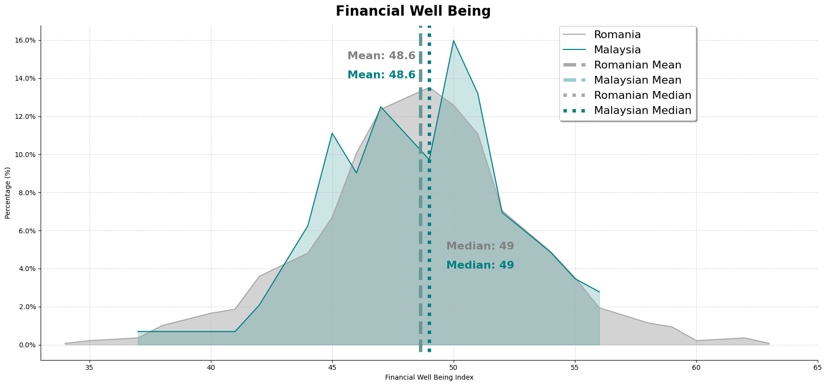
Based on the results, we can observed that the financial well being of both dataset. Romania has a wider range of scores as well as looking normally distributed. Our dataset might be suffering from insufficient data, which is causing the irregular shape.
We can also observe that there are about the same percentage of people experiencing the same amount of financial well being. Furthermore, for the romanian dataset, there are accounts of above 60 while our malaysian dataset, have not scored anything about 60. Furthermore, the mean line for both of the data are identical.
Having seen that our dataset's financial literacy is higher than the romanian dataset, and having more higher earners, we would expect that the financial well being of our dataset should be higher as well. However, we can observe that the maximum score for financial well being does not even pass 57.5.
# Score Aggregation
# ==================

# To store the romanian column indexes
romanian_financial_well_being_columns = []

# Base string is A1 and B1
base_string = ['A1_', 'B1_']

# Print romanian columns to see
print(romanian_dataset.columns)

# Loop from 1 to 6, for base string A
for sub_string in range(1,7):
    romanian_financial_well_being_columns.append(
        base_string[0] + str(sub_string)
    )

# Loop from 1 to 4, for base string B
for sub_string in range(1,5):
    romanian_financial_well_being_columns.append(
        base_string[1] + str(sub_string)
    )

# Too many strings will be required, therefore
# Check for the columns required
for num, column in enumerate(our_columns):
    if num > 45 or num < 25:
        continue
    else:
        print( str(num) + '\t' + column)

# Store the required colum
our_financial_well_being_columns = []

for num in range(31, 42):
    if num != 37:
        our_financial_well_being_columns.append(num)

# Completely = 4
completely_is_4 = [0, 1, 3]
completely_is_4_dict = {
    'Completely': 4,
    'Very well': 3,
    'Somewhat': 2,
    'Very little': 1,
    'Not at all': 0
}

# Completely = 0
completely_is_0 = [2, 4, 5]
completely_is_0_dict = {
    'Completely': 0,
    'Very well': 1,
    'Somewhat': 2,
    'Very little': 3,
    'Not at all': 4
}

# Always = 0
always_is_0 = [6, 8, 9]
always_is_0_dict = {
    'Always': 4,
    'Often': 3,
    'Often ': 3,
    'Sometimes': 2,
    'Rarely': 1,
    'Never':  0
}

# Always = 4
always_is_4 = [7]
always_is_4_dict = {
    'Always': 0,
    'Often': 1,
    'Often ': 1,
    'Sometimes': 2,
    'Rarely': 3,
    'Never':  4
}

# For romanian dataset

# Initialize lists to store column
romanian_financial_well_being_columns_completely_is_4 = []
romanian_financial_well_being_columns_completely_is_0 = []
romanian_financial_well_being_columns_always_is_4 = []
romanian_financial_well_being_columns_always_is_0 = []

# Loop through the list to get the columns
for num in completely_is_4:
    romanian_financial_well_being_columns_completely_is_4.append(
        romanian_financial_well_being_columns[num]
    )

for num in completely_is_0:
    romanian_financial_well_being_columns_completely_is_0.append(
        romanian_financial_well_being_columns[num]
    )

for num in always_is_0:
    romanian_financial_well_being_columns_always_is_0.append(
        romanian_financial_well_being_columns[num]
    )

for num in always_is_4:
    romanian_financial_well_being_columns_always_is_4.append(
        romanian_financial_well_being_columns[num]
    )

# Converting the values
romanian_financial_well_being = \
    romanian_dataset[
        romanian_financial_well_being_columns_completely_is_4
    ].replace(completely_is_4_dict)

romanian_financial_well_being[romanian_financial_well_being_columns_completely_is_0] = \
    romanian_dataset[
        romanian_financial_well_being_columns_completely_is_0
    ].replace(completely_is_0_dict)

romanian_financial_well_being[romanian_financial_well_being_columns_always_is_4] = \
    romanian_dataset[
        romanian_financial_well_being_columns_always_is_4
    ].replace(always_is_4_dict)

romanian_financial_well_being[romanian_financial_well_being_columns_always_is_0] = \
    romanian_dataset[
        romanian_financial_well_being_columns_always_is_0
    ].replace(always_is_0_dict)

# For our dataset

# Initialize lists to store column
our_financial_well_being_columns_completely_is_4 = []
our_financial_well_being_columns_completely_is_0 = []
our_financial_well_being_columns_always_is_4 = []
our_financial_well_being_columns_always_is_0 = []

# Loop through the list to get the columns
for num in completely_is_4:
    our_financial_well_being_columns_completely_is_4.append(
        our_columns[our_financial_well_being_columns[num]]
    )

for num in completely_is_0:
    our_financial_well_being_columns_completely_is_0.append(
        our_columns[our_financial_well_being_columns[num]]
    )

for num in always_is_0:
    our_financial_well_being_columns_always_is_0.append(
        our_columns[our_financial_well_being_columns[num]]
    )

for num in always_is_4:
    our_financial_well_being_columns_always_is_4.append(
        our_columns[our_financial_well_being_columns[num]]
    )

# Converting the values
our_financial_well_being = \
    our_dataset[
        our_financial_well_being_columns_completely_is_4
    ].replace(completely_is_4_dict)

our_financial_well_being[our_financial_well_being_columns_completely_is_0] = \
    our_dataset[
        our_financial_well_being_columns_completely_is_0
    ].replace(completely_is_0_dict)

our_financial_well_being[our_financial_well_being_columns_always_is_4] = \
    our_dataset[
        our_financial_well_being_columns_always_is_4
    ].replace(always_is_4_dict)

our_financial_well_being[our_financial_well_being_columns_always_is_0] = \
    our_dataset[
        our_financial_well_being_columns_always_is_0
    ].replace(always_is_0_dict)

financial_well_being_index_dict = {
    0 : 14,
    1 : 19,
    2 : 22,
    3 : 25,
    4 : 27,
    5 : 29,
    6 : 31,
    7 : 32,
    8 : 34,
    9 : 35,
    10: 37,
    11: 38,
    12: 40,
    13: 41,
    14: 42,
    15: 44,
    16: 45,
    17: 46,
    18: 47,
    19: 49,
    20: 50,
    21: 51,
    22: 52,
    23: 54,
    24: 55,
    25: 56,
    26: 58,
    27: 59,
    28: 60,
    29: 62,
    30: 63,
    31: 65,
    32: 66,
    33: 68,
    34: 69,
    35: 71,
    36: 73,
    37: 75,
    38: 78,
    39: 81,
    40: 86
}

# Romanian Dataset
# Create a column that takes the sum of all the other columns
romanian_financial_well_being['Score'] = \
    romanian_financial_well_being[romanian_financial_well_being_columns]\
        .sum(axis=1)

# Given the current score, map it to the financial well being score
romanian_financial_well_being['Financial Well Being Index'] =\
    romanian_financial_well_being['Score']\
        .map(financial_well_being_index_dict)

# Storing Financial Well Being Index into main dataset
romanian_dataset['Financial Well Being Index'] = romanian_financial_well_being['Financial Well Being Index']

# Our Dataset
# Create a column that takes the sum of all the other columns
our_financial_well_being['Score'] = \
    our_financial_well_being[
        our_columns[our_financial_well_being_columns]
    ].sum(axis=1)

# Given the current score, map it to the financial well being score
our_financial_well_being['Financial Well Being Index'] = \
    our_financial_well_being['Score']\
        .map(financial_well_being_index_dict)

# Storing the Financial Well Being Index into the main dataset
our_dataset['Financial Well Being Index'] = our_financial_well_being['Financial Well Being Index']

# Data Preparation
# ================
# Get unique values of the financial well being index, and sort them in ascending order
# The plot will get wonky if it is not in order
romanian_financial_well_being_x = \
    np.sort(romanian_financial_well_being['Financial Well Being Index'].unique())\

our_financial_well_being_x = \
    np.sort(our_financial_well_being['Financial Well Being Index'].unique())

# Get the value count of each score, and then divide it by the size of each dataset
romanian_financial_well_being_y = \
    (romanian_financial_well_being['Financial Well Being Index']\
        .value_counts().get(romanian_financial_well_being_x)\
        / len(romanian_financial_well_being))

our_financial_well_being_y = \
    (our_financial_well_being['Financial Well Being Index']\
        .value_counts().get(our_financial_well_being_x)\
        / len(our_financial_well_being)
    )

# Get mean value of the financial well being index
romanian_financial_well_being_mean = romanian_financial_well_being['Financial Well Being Index'].mean()
our_financial_well_being_mean = our_financial_well_being['Financial Well Being Index'].mean()

# Get median value of the financial well being index
romanian_financial_well_being_median = romanian_financial_well_being['Financial Well Being Index'].median()
our_financial_well_being_median = our_financial_well_being['Financial Well Being Index'].median()

# Get the std value of the financial well being index
romanian_financial_well_being_std = romanian_financial_well_being['Financial Well Being Index'].std()
our_financial_well_being_std = our_financial_well_being['Financial Well Being Index'].std()

# Initialize the figure
figure, ax = plt.subplots(figsize=(17,8))
figure.suptitle(
    'Financial Well Being',
    fontweight = 'bold',
    fontsize = 20
    )

# Plot romania data
# ==================
ax.plot(
    romanian_financial_well_being_x,
    romanian_financial_well_being_y,
    color = 'darkgray',
    label = 'Romania'
)

ax.fill_between(
    romanian_financial_well_being_x,
    romanian_financial_well_being_y[romanian_financial_well_being_x],
    alpha = 0.5,
    color = 'darkgray'
)

# Plot our data
# ===============
ax.plot(
    our_financial_well_being_x,
    our_financial_well_being_y,
    color = 'teal',
    label = 'Malaysia'
)

ax.fill_between(
    our_financial_well_being_x,
    our_financial_well_being_y[our_financial_well_being_x],
    alpha = 0.2,
    color = 'teal'
)

# Mean line and annotations
# ==========================
ax.axvline(
    romanian_financial_well_being_mean,
    0.025,
    ls = '--',
    color = 'darkgray',
    label = 'Romanian Mean',
    linewidth =  5
)

ax.annotate(
    f'Mean: {romanian_financial_well_being_mean:.3g}',
    xy=(romanian_financial_well_being_mean - 3, 0.15),
    fontsize=16, fontweight='bold', color='grey'
)

ax.axvline(
    our_financial_well_being_mean,
    0.025,
    ls = '--',
    color = 'teal',
    label = 'Malaysian Mean',
    alpha = 0.4,
    linewidth =  5
)

ax.annotate(
    f"Mean: {our_financial_well_being_mean:.3g}",
    xy=(our_financial_well_being_mean - 3 ,0.14),
    fontsize=16, fontweight='bold', color='teal')

# Median line and annotations
# ==========================
ax.axvline(
    romanian_financial_well_being_median,
    0.025,
    ls = ':',
    color = 'darkgray',
    label = 'Romanian Median',
    linewidth = 5
)

ax.annotate(
    f"Median: {romanian_financial_well_being_median:.3g}",
    xy=(romanian_financial_well_being_median + 0.7 ,0.05),
    fontsize=16, fontweight='bold', color='grey')

ax.axvline(
    our_financial_well_being_median,
    0.025,
    ls = ':',
    color = 'teal',
    label = 'Malaysian Median',
    linewidth = 5
)

ax.annotate(
    f"Median: {our_financial_well_being_median:.3g}",
    xy=(our_financial_well_being_median + 0.7 ,0.04),
    fontsize=16, fontweight='bold', color='teal')

# Set the x limit, initially used 16 to 91, the limits of the financial well being score, but the plot will look thin
ax.set_xlim(33,65)

# Set x and y label and have a larger legend
ax.set_ylabel('Percentage (%)')
ax.set_xlabel('Financial Well Being Index')
ax.spines[['top', 'right']].set_visible(False)
ax.legend(fontsize = 16, shadow=True, bbox_to_anchor=(0.85, 1.015))
formatter = mtick.PercentFormatter(xmax=1.0)
ax.yaxis.set_major_formatter(formatter)
ax.grid(alpha=0.5, linestyle='--')

# Optimize layout and show the figure
plt.tight_layout()
plt.show()
Invested Money in any Financial Instruments
For the romanian dataset, the following table is what the each column represent. We will only be changing the 'yes' and 'no' to 0s and 1s, and create a custom dictionary for labeling the columns.
For the romanian dataset, the following table are the options available for them to choose. They were only able to pick 2 out of the listed choices.
| Column | Financial Instrument |
|---|---|
| I2_1 | Savings deposit |
| I2_2 | Stocks |
| I2_3 | Bonds |
| I2_4 | Real estate |
| I2_5 | Investment funds |
| I2_6 | Life insurance |
| I2_7 | Cryptocurrency |
| I2_8 | I saved and kept money at home |
| I2_0 | I have not saved or invested |
For our dataset and our survey, we have allowed our participants to select whichever is applicable to them, because it is likely to be holding more than 2 choices shown. Additionally, we added more choices of financial instruments, as well as altering one from the ones from the romanian dataset. The additional and alterned choice are as follows:
| Financial Instrument |
|---|
| Life Insurance --> Investment-linked Insurance |
| Sport Betting |
| Foreign Exchange (Forex) |
| Futures |
| Others |
We changed 'Life Insurance' to 'Investement-linked Insurance', because the life insurance schemes here are not really viewed as choices of investement, but a financial protection from accidents. However, there are insurance coverages, including life insurances, that has some form of investment component or feature that comes along with it. Hence, the change of the choice for better clarification.
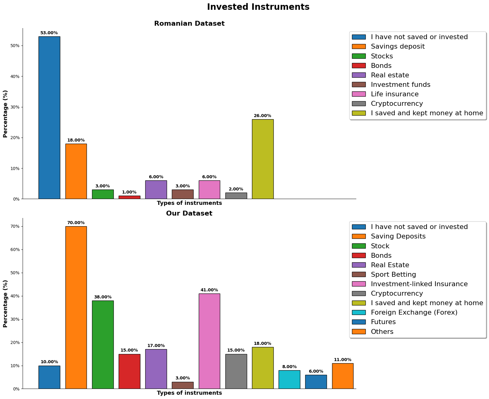
We can see a drastic difference in the saving habits from our dataset and the romanian dataset, just from the first 2 choices alone. There is only 10% of the our dataset who have not saved and have not invested while there were half of the romanian dataset who does the same. Almost everyone in our dataset has at least got a savings deposit while the romanian dataset has 18%.
# Data Preparation
# =================

# Romanian Dataset ===
# To store the column indexes
romanian_invested_instruments_columns = []

# Base string is I2_
romanian_invested_instruments_string = 'I2_'

# Loop from 0 to 8
for sub_string in range(0,9):

    # Store the base string and sub string into the list
    romanian_invested_instruments_columns.append(
        romanian_invested_instruments_string +
        str(sub_string)
    )

# Custom dictionary to represent the labels in plot
custom_dict_invested_instruments_romanian_columns = {

    'I2_0': 'I have not saved or invested',
    'I2_1': 'Savings deposit',
    'I2_2': 'Stocks',
    'I2_3': 'Bonds',
    'I2_4': 'Real estate',
    'I2_5': 'Investment funds',
    'I2_6': 'Life insurance',
    'I2_7': 'Cryptocurrency',
    'I2_8': 'I saved and kept money at home'

}

# Changing the 'yes' and 'no' values into binary
romanian_invested_instruments = romanian_dataset[romanian_invested_instruments_columns]\
    .replace({'Yes':1 , 'No':0})

# Storing new names for the processed columns
processed_columns = []
base_string = 'Saved or Invested in '
for col in romanian_invested_instruments_columns:
    processed_columns.append(
        base_string +
        custom_dict_invested_instruments_romanian_columns[col])

# Store the new processed columns into main dataset
romanian_dataset[processed_columns] = romanian_invested_instruments

# Our Dataset ==

# Get the column string
our_invested_instruments_string = getOurString('saved or invested money', our_columns)

# Split each row as it contains multiple entries
our_invested_instruments = our_dataset[our_invested_instruments_string]\
    .str.split(',', expand=True).stack()

# Take the values and turn it into columns, and fill the blanks with 0s
our_invested_instruments = pd.get_dummies(our_invested_instruments)\
    .groupby(level=0).sum()

# Print the columns for custom dict
print('Columns: ', our_invested_instruments.columns)

# Custom dictionary to arrange the columns similar to the above
custom_dict_invested_instruments_our_columns = {

    0:'I have not saved or invested',
    1:'Saving Deposits',
    2:'Stock',
    3:'Bonds',
    4:'Real Estate',
    5:'Sport Betting',
    6:'Investment-linked Insurance',
    7:'Cryptocurrency',
    8:'I saved and kept money at home',
    9:'Foreign Exchange (Forex)',
    10:'Futures',
    11:'Others'

}

# Processed column names
processed_columns = 'Saved or Invested in ' + our_invested_instruments.columns

# Store into main dataset
our_dataset[processed_columns] = our_invested_instruments

# Plot Figure
# =============
# Initialize figure
fig, ax = plt.subplots(2,1,figsize=(17,13))

# Insert Title
fig.suptitle(
    'Invested Instruments',
    fontweight = 'bold',
    fontsize = 20, y=1)

# Set width
width = 0.8

# Set formatter for percentage
formatter = mtick.PercentFormatter(xmax=1.0)

datasets = [
    ('Romanian Dataset', romanian_invested_instruments_columns, romanian_invested_instruments, custom_dict_invested_instruments_romanian_columns, ax[0]),
    ('Our Dataset', our_invested_instruments, custom_dict_invested_instruments_our_columns, custom_dict_invested_instruments_our_columns, ax[1])
]

for set, columns, dict_cols, labels, ax in datasets:

    if set == 'Romanian Dataset':
        for col_no, column in enumerate(columns):

            container = ax.bar(
                col_no, round(dict_cols[column].mean(),2),
                width, label=labels[column], edgecolor='black'
            )

            ax.bar_label(container, fontsize=10, fontweight='bold', padding=3, fmt='{:.2%}')
    else:
        for col_no in range(0, len(columns.columns)):

            container = ax.bar(
                col_no, round(columns[dict_cols[col_no]].mean(),2),
                width, label=labels[col_no], edgecolor='black'
            )

            ax.bar_label(container, fontsize=10, fontweight='bold', padding=3, fmt='{:.2%}')

    ax.set_title(set, fontsize=16, fontweight='bold')
    ax.set_xticks([])
    ax.set_ylabel('Percentage (%)', fontsize=13, fontweight='bold')
    ax.set_xlabel('Types of instruments', fontsize=13, fontweight='bold')
    ax.set_xlim(-1, 11.5)
    ax_distict_legends = ax.get_legend_handles_labels()[1][:]
    ax.legend(ax_distict_legends, bbox_to_anchor=(1.4,1), shadow=True, fontsize=16)
    ax.yaxis.set_major_formatter(formatter)
    ax.spines[['right', 'top']].set_visible(False)

plt.tight_layout()
plt.show()
Financial Decision Influence
Similarly to the above, we have added more options for participants to choose, so we can further explore.
For the romanian dataset, the following is the choices given:
| Column | Financial Decision Influence |
|---|---|
| I3_1 | Mass-media (TV and radio) |
| I3_2 | Online and printed newspapers |
| I3_3 | Financial websites and mobile apps |
| I3_4 | Advice from friends |
| I3_5 | Personal experience and knowledge |
| I3_6 | Other sources |
For our dataset, we have added the following as well:
| Financial Decision Influence |
|---|
| Social Media |
| Advice from Family |
| Financial Advisor |
Initially, we thought of plotting the likert scale from least value to highest value for every source but it looked too messy to comprehend. Therefore, chose to only filter those that have values of 3 and 4, which are 'very influenced' and 'main influence' respectively, and to display them as percentage basis.
Because of the lesser restriction in our survey, participants get to rank how they feel about each of the source. We can see that many values are inflated and might need a deeper dive and specify what to filter and look into. The initial draft of the survey, we wanted the survey participants to rank their top 4 influences, but there were feedback stating that it was too confusing to do, so we then changed it too ranking all of them, but then there were more feedback about it being tedious as well. Hence, we ended up having them choose how influential each source are to them.
We can observe that for the romanian dataset, due to the limitation of choice, their answer should be more substantiated and for them, there are heavily influence by mass-media and from learning from their own personal experience and knowledge, while for our dataset, many of the participants are heavily influenced by social media and advice from family.
As shown by the result, even though 27% of them chose other as the source, but there were only few entries of proper input. It could be because of the survey design, participants might have been confused or selected wrongly.
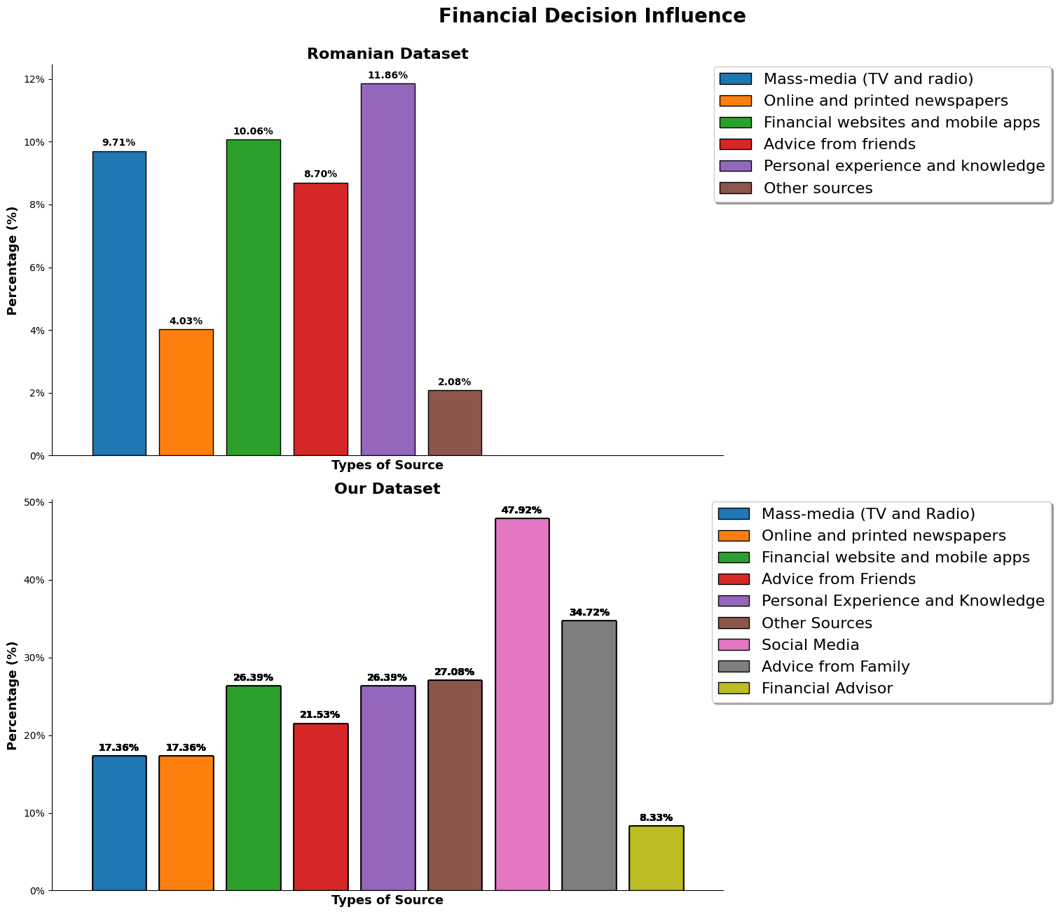
When, we look into 'other sources', the listed output were 'Financial Database', 'Financial Books', and 'Constultant'.
# Data Prepration
# ===============

# Romanian Dataset ==
# To store the column indexes
romanian_financial_decision_columns = []

# Base string is I3
romanian_financial_decision_string = 'I3_'

# Loop from 1 to 6
for sub_string in range(1,7):

    romanian_financial_decision_columns.append(
        romanian_financial_decision_string +
        str(sub_string)
    )

# Custom dictionary to represent the labels in plot
custom_dict_financial_decision_romanian_columns = {

    'I3_1':'Mass-media (TV and radio)',
    'I3_2':'Online and printed newspapers',
    'I3_3':'Financial websites and mobile apps',
    'I3_4':'Advice from friends',
    'I3_5':'Personal experience and knowledge',
    'I3_6':'Other sources'

}

# Changing the 'yes' and 'no' values into binary
romanian_financial_decisions = romanian_dataset[romanian_financial_decision_columns]\
    .replace({'Yes':1, 'No':0})

# Filling the null values
for col in romanian_financial_decision_columns:
    romanian_financial_decisions[col] = romanian_financial_decisions[col].fillna(0)

# Names for the processed columns
romanian_financial_decision_columns_processed = []
for col in romanian_financial_decision_columns:

    romanian_financial_decision_columns_processed.append(
        'Financial Decision: ' +
        custom_dict_financial_decision_romanian_columns[col]
    )

# Store them into main dataset
romanian_dataset[romanian_financial_decision_columns_processed] = romanian_financial_decisions

# Our Dataset ===
# Store the required
our_financial_decision_columns = [x for x in range(16, 25)]

# Store the index of the column, column description and match the order to the romanian dataset
custom_dict_financial_decision_our_columns = {

    0:( 16, 'Mass-media (TV and Radio)'),
    1:( 17, 'Online and printed newspapers'),
    2:( 18, 'Financial website and mobile apps'),
    3:( 20, 'Advice from Friends'),
    4:( 22, 'Personal Experience and Knowledge'),
    5:( 24, 'Other Sources'),
    6:( 19, 'Social Media'),
    7:( 21, 'Advice from Family'),
    8:( 23, 'Financial Advisor')

}

# Convert the string input into integers
our_financial_decision = our_dataset[our_columns[our_financial_decision_columns]]\
    .replace({
        'Not applicable / No influence at all': 0,
        'Somewhat influenced': 1,
        'Influenced': 2,
        'Very Influenced': 3,
        'Main influence': 4
    })

# Filling some of the null values
our_financial_decision = our_financial_decision.fillna(0)

# Renaming the processed columns
our_financial_decision_column_name = []
for col in our_financial_decision.columns:
    print('Financial Decision: ' + col[6:])
    our_financial_decision_column_name.append('Financial Decision: ' + col[6:])

# Store the processed columns into the main dataset
our_dataset[our_financial_decision_column_name] = our_financial_decision

# Plot Figure
# ===========
# Initialize the figure
figure, ax = plt.subplots(2,1, figsize=(17,13))
figure.suptitle(
    'Financial Decision Influence',
    fontsize = 20,
    fontweight = 'bold', y=1)

# Set width
width = 0.8

# Set formatter for percentage
formatter = mtick.PercentFormatter(xmax=1.0)

# Set values to loop
datasets = [
    ('Romanian Dataset', ax[0]),
    ('Our Dataset', ax[1])
]

# Looping through values
for set, ax in datasets:
    if set == 'Romanian Dataset':
        for col_no, column in enumerate(romanian_financial_decision_columns):
            container = ax.bar(
                col_no, romanian_financial_decisions[column].mean(),
                width = width, label = custom_dict_financial_decision_romanian_columns[column],
                edgecolor = 'black'
            )

            ax.bar_label(container, fontsize=10, fontweight='bold', padding=3, fmt='{:.2%}')
    else:
        for col_no in range(0, len(our_financial_decision_columns)):
            container = ax.bar(
                col_no,
                our_financial_decision[
                    our_columns[our_financial_decision_columns[col_no]]]\
                        .loc[(our_financial_decision[
                            our_columns[our_financial_decision_columns[col_no]]] > 2)]\
                                .count()/our_financial_decision.count(),
                width = width,
                label = custom_dict_financial_decision_our_columns[col_no][1],
                edgecolor = 'black'
            )

            ax.bar_label(container, fontsize=10, fontweight='bold', padding=3, fmt='{:.2%}')

    # Styling
    ax.set_xticks([])
    ax.set_title(set, fontweight='bold', fontsize=16)
    ax.set_ylabel('Percentage (%)', fontsize=13, fontweight='bold')
    ax.set_xlabel('Types of Source', fontsize=13, fontweight='bold')
    ax.set_xlim(-1, 9)
    ax_distict_legends = ax.get_legend_handles_labels()[1][:]
    ax.legend(ax_distict_legends, bbox_to_anchor=(1.5,1.015), fontsize=16, shadow=True)
    ax.yaxis.set_major_formatter(formatter)
    ax.spines[['top', 'right']].set_visible(False)

# Optimize layout and show figure
plt.tight_layout()
plt.show()
Exploring and Futher Analysing Combined Traits
Gender accross Age Bin
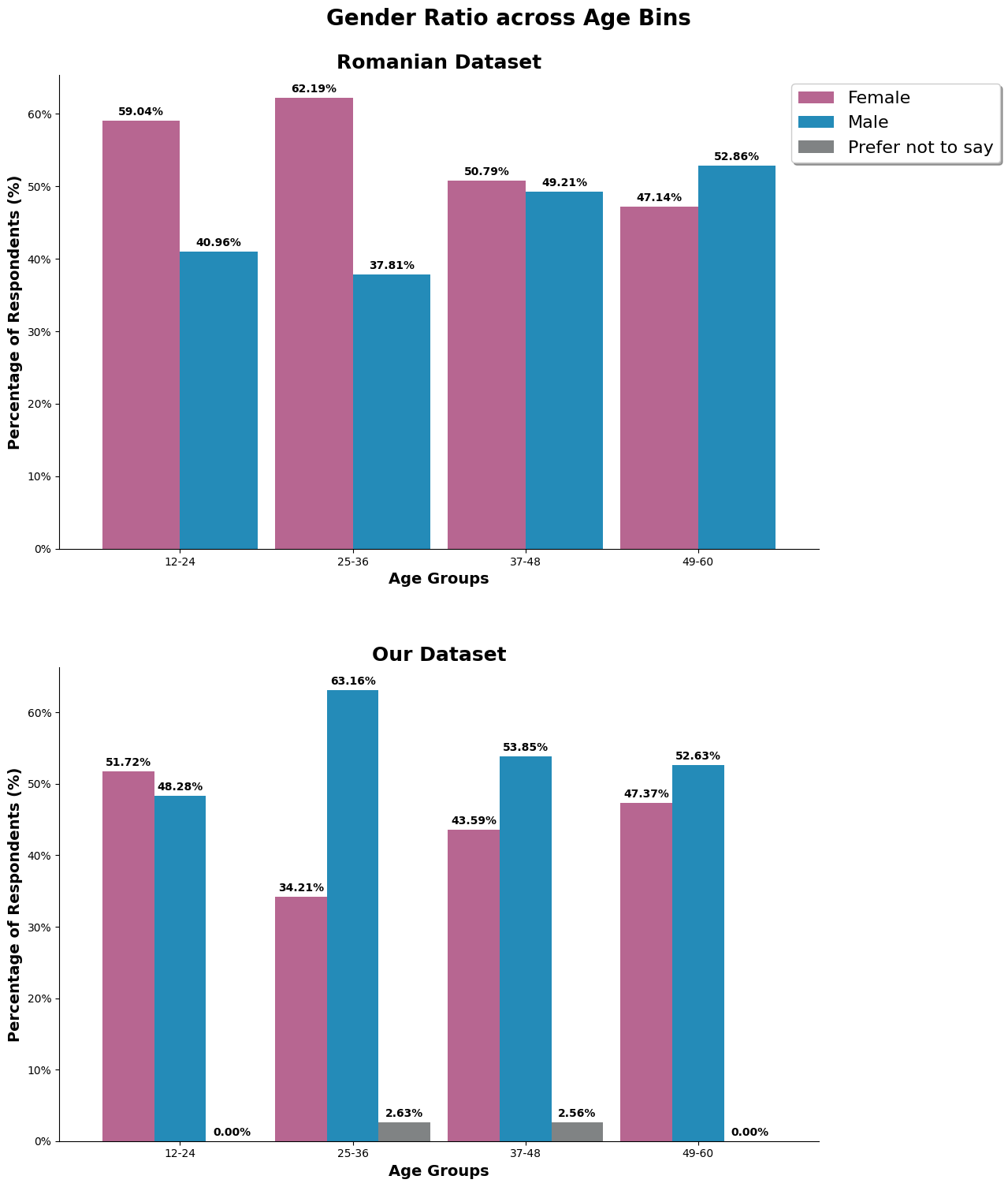
Digging deeper into gender and split it by the age groups, we can observe the causes of the imbalance ratio of gender in our dataset. It is very male dominant at the age range, two times more than female. Additionally, this is also the age group where there is alot of survey participants.
For the romanian dataset, the first two age group has a slightly of females, but because the first two age group makes ups lesser portion of the population, it has a lesser effect on the overall gender ratio.
# Get the age and gender columns from the data set
romanian_dataset_age_gender = romanian_dataset.filter(items=['SD2', 'SD3'])

our_age_string = getOurString('your age', our_columns)
our_dataset_age_gender = our_dataset.filter(
    items = [
        our_age_string,
        our_gender_string
    ]
)

# Segment and sort data in to bins
age_bins_romania = pd.cut(
    romanian_dataset_age_gender['SD3'],
    bins = [x for x in range(12,61,12)],
    labels = ['12-24', '25-36', '37-48', '49-60'])

age_bins_our = pd.cut(
    our_dataset_age_gender[our_age_string],
    bins = [x for x in range(12,61,12)],
    labels = ['12-24', '25-36', '37-48', '49-60']
)

# Group the data based on Age
gender_ratio_romania = romanian_dataset_age_gender.groupby(age_bins_romania, observed=False)['SD2'].value_counts(normalize=True)
gender_ratio_our = our_dataset_age_gender.groupby(age_bins_our, observed=False)[our_gender_string].value_counts(normalize=True)

# Initialize the figure with subplots
fig, (ax1, ax2) = plt.subplots(2, 1, figsize=(13, 15))
fig.suptitle('Gender Ratio across Age Bins',
             fontweight = 'bold', size = 20, y = 1)

# Set color list
color = ["#B76691", "#248BB8", "#808384"]

# Set dataset and values
datasets = [
    (gender_ratio_romania, 'Romanian Dataset', 'darkgray', ax1),
    (gender_ratio_our, 'Our Dataset', 'teal', ax2)
]
formatter = mtick.PercentFormatter(xmax=1.0)

# Loop dataset and plot the bars
for dataset, title, title_color, ax in datasets:
    dataset.unstack().plot(kind='bar',ax=ax, color=color, width=0.9, rot=0)
    for c in ax.containers:
        ax.bar_label(c, fmt='{:.2%}', fontweight='bold', fontsize=10, padding=3)

    ax.set_title(title, fontsize=18, fontweight='bold')
    ax.set_ylabel('Percentage of Respondents (%)', fontweight='bold', fontsize=14)
    ax.set_xlabel('Age Groups', fontweight='bold', fontsize=14)
    ax.legend().remove()
    ax.spines[['top', 'right']].set_visible(False)
    ax.yaxis.set_major_formatter(formatter)

plt.legend(bbox_to_anchor=(1.25,2.25), loc='upper right', shadow=True, fontsize=16)
plt.tight_layout()
plt.subplots_adjust(hspace=0.25)
plt.show()
Income based on other factors
Income across Age Groups - Does income come with age?

The graph shows income across the age groups without normalization. We can observe that even at the age group of '25 - 36', our dataset already consists of 10 respondents (about 7% of our dataset) that is earning above RM9999.
While the graph for romanian dataset, seems to be normally distributed and shaped according to the age group graph in the section above.
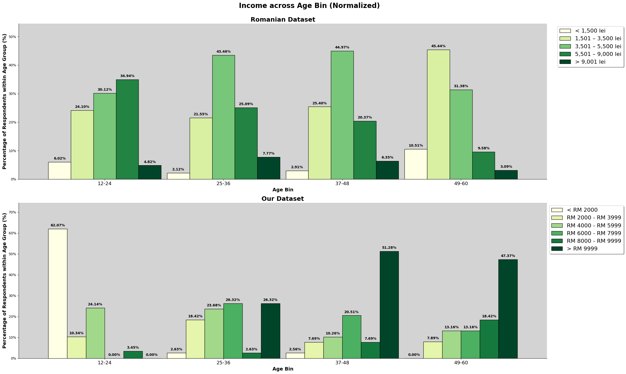

This later two graphs above shows the normalized values for the first graph above. One has trend lines and one does not. The trend lines help visualize and guide us to identify any trends.
The difference in the shape of the graph is minimal for our dataset. However, we can observe that the older the age group, the more high earners ('RM8000 - RM9999' and '>RM9999') there are. Additionally, we also see the other income ranges below 'RM7999', shrink as the age group increases, which supports the idea that the older we get, the more promotions and bonuses we get, so as our income.
For the romanian dataset, we see shrinkage for those that make '5501 - 9000' as the older the age group, but there is an increase in those that make '1501 - 3500'. Even for '1500', we see it trend downwards, but increase in the last age group. This might be because romanian still work after the retirement age, or move on to lower stress jobs as they get older.
Income across Education Attainment - Does it pay to have a higher education?
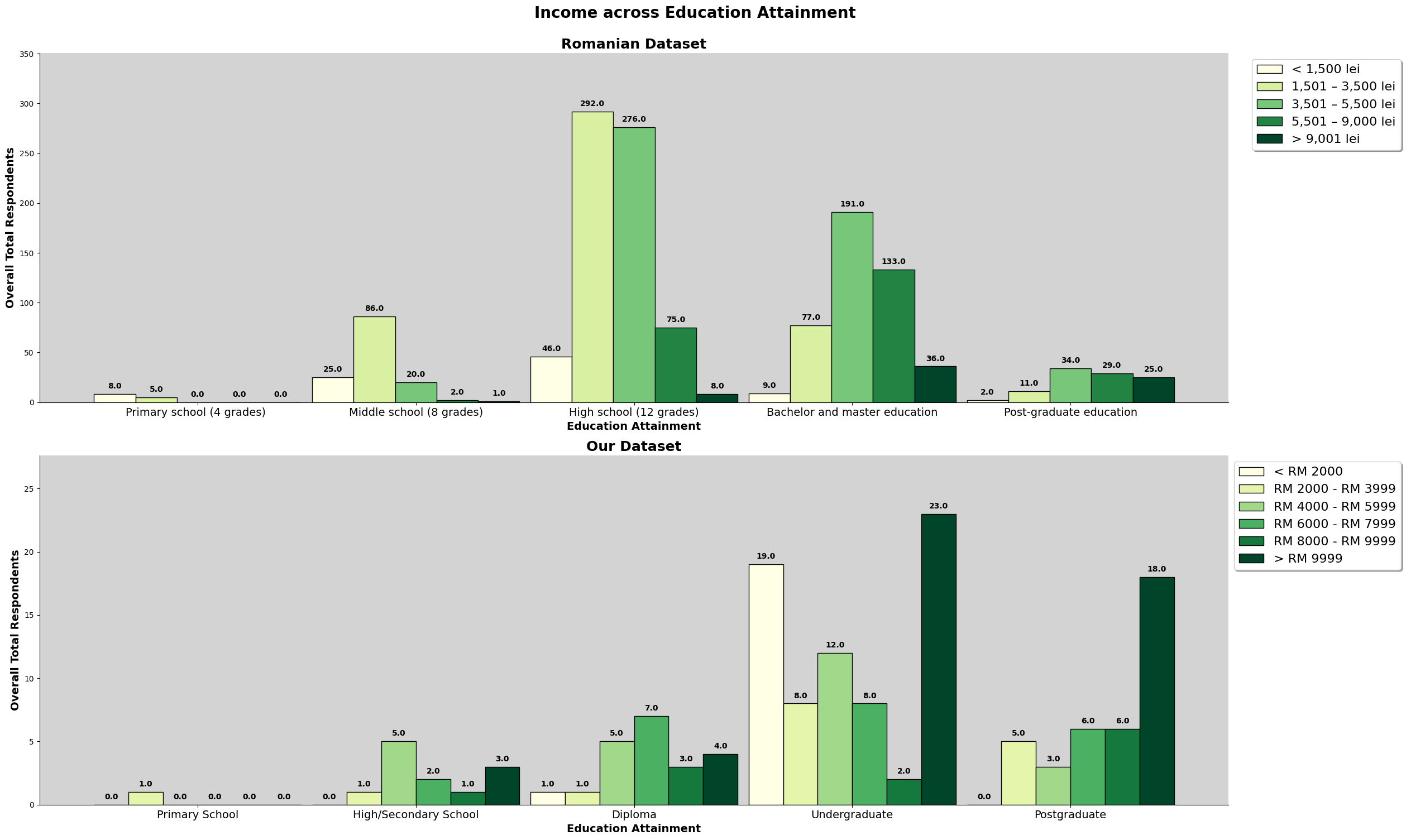
The graph shows income across the education attainment levels of each dataset, without normalization. We can observe that the education attainment group with the most population, a wider range of income range groups. Hence, we need to normalize to make any statement on the observations.
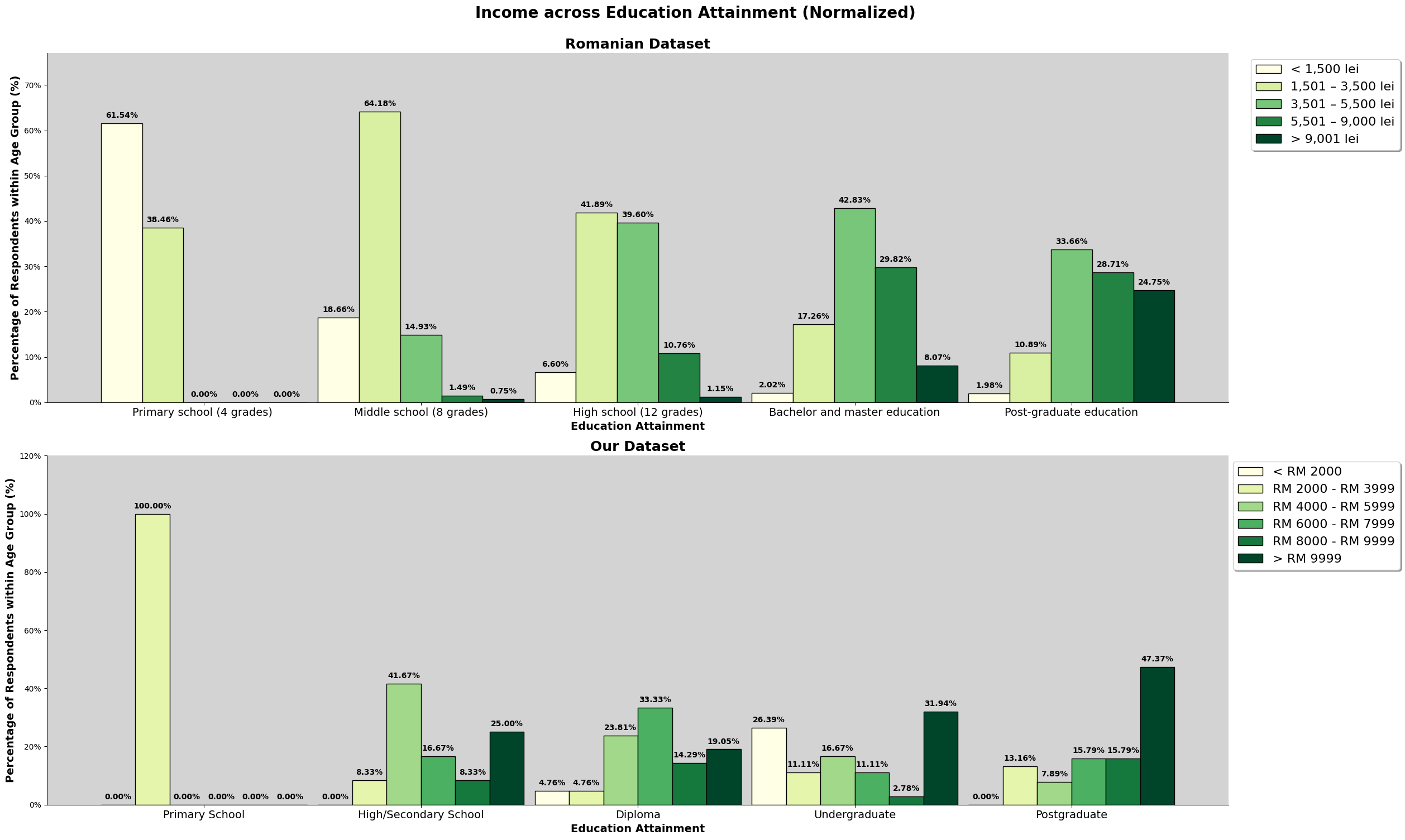
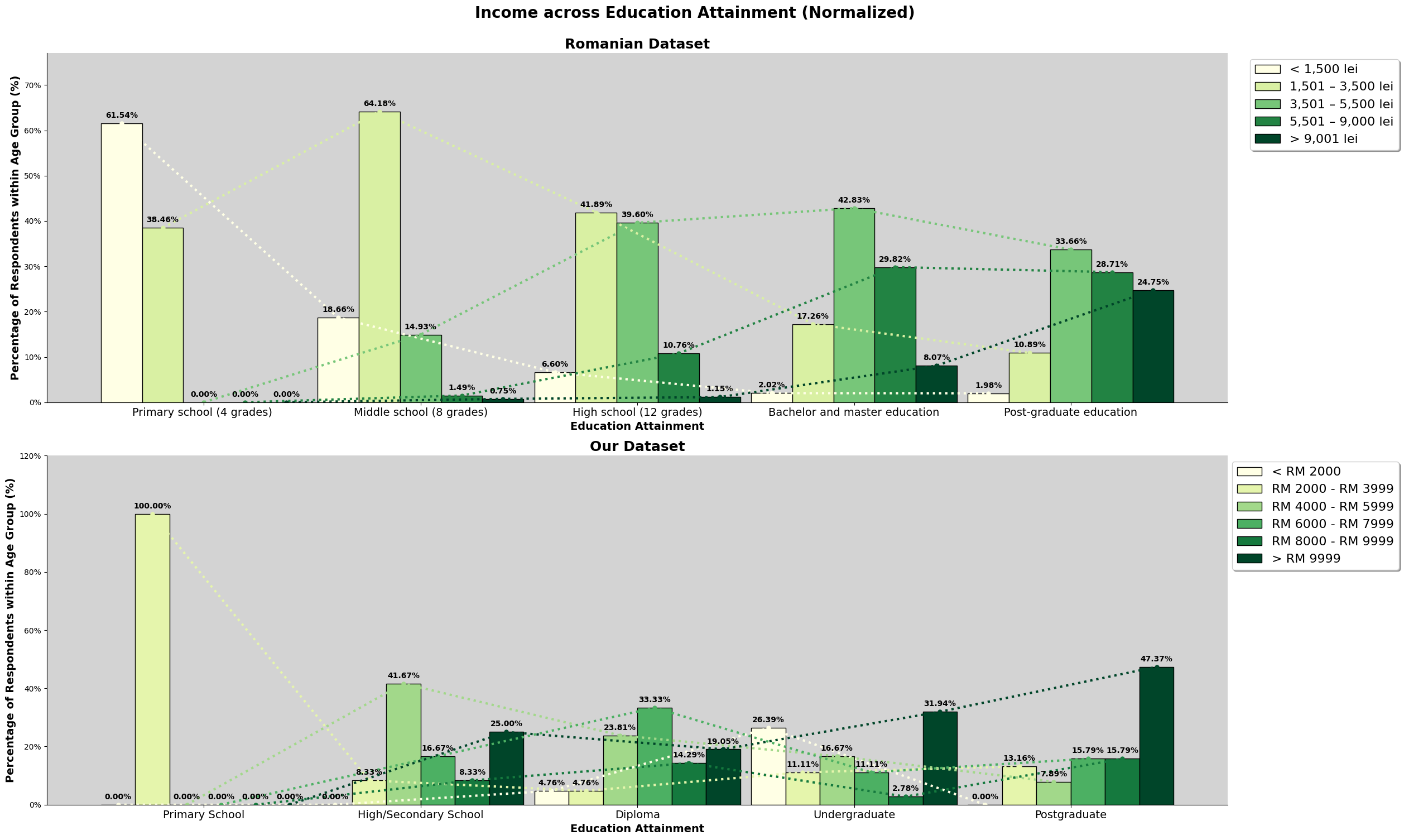
Once normalized, as shown in the above two graphs, we can observe that in the romanian dataset, that the lowest income range, trends downward as education attainment is higher. This is also applicable to income range '1501 - 3500 lei', where other than seeing an increase from 'Primary School' to 'Middle School', this income range also trend downwards as an individual have a higher education attainment. The remaining income ranges, all increase according to education attainment.
For our dataset, we can also see that there is an increase in highest earners as education attainment increases. However, there is a sudden spike in the income range '< RM2000' in the 'undergraduate' group is due having higher number of younger inidviduals, which either are fresh graudates or going through their internships.
Both dataset do show data that supports the claim that having higher education, does lead to having higher income.
Income vs Gender - Is the gender pay gap real?

This current graph shows the income range between two genders for both dataset, without normalization. For the romanian dataset the income differences are about the same, except for the income range of '5501 - 9000 lei', where there are almost 30 more females. However, the dataset does consists of more females. As for our dataset, we can clearly see that there are a lot of males there are in the '>RM9000' income range. Similarly, we need to take note that that is also because there are more males in our dataset.

After normalizing, we can observe that for the romanian dataset, there are almost no difference between the both males and female. For our dataset, the normalization did not change the context much, as our dataset might be too 'male-biased'. We see that 40% of those that are male, are in the income range of '>RM9000'.
Therefore, there is no gender pay gap shown in the romanian dataset but there is with our dataset.
# Set column string
our_income_string = getOurString('income', our_columns)
romanian_income_string = 'SD7'

# Create a custom dictionary to map
custom_dict_romania_income = {
    '< 1,500 lei': 0,
    '1,501 – 3,500 lei': 1,
    '3,501 – 5,500 lei': 2,
    '5,501 – 9,000 lei': 3,
    '> 9,001 lei': 4
}
custom_dict_our_income = {
    '< RM 2000':0,
    'RM 2000 - RM 3999':1,
    'RM 4000 - RM 5999':2,
    'RM 6000 - RM 7999':3,
    'RM 8000 - RM 9999':4,
    '> RM 9999':5,
}

# Set the custom order to the column
romanian_dataset[romanian_income_string] = romanian_dataset[romanian_income_string].astype(pd.CategoricalDtype(
    categories=custom_dict_romania_income, ordered=True))

our_dataset[our_income_string] = our_dataset[our_income_string].astype(pd.CategoricalDtype(
    categories=custom_dict_our_income, ordered=True
))

# Function to create an income graph based on columns provided
def create_income_graph(our_column, romanian_column, title:str, normalize:bool=False, lineplot:bool=False,
                        our_dataset=our_dataset, romanian_dataset=romanian_dataset):

    # Data Preparation
    # =================
    romanian_df = romanian_dataset[[romanian_column, romanian_income_string]].groupby(romanian_column, observed=False)\
        .value_counts(normalize=normalize)
    our_df = our_dataset[[our_column, our_income_string]].groupby(our_column, observed=False)\
        .value_counts(normalize=normalize)

    # Plot Figure
    # ============
    # Initialize figure
    fig, (ax1, ax2) = plt.subplots(2, 1, figsize=(25,15) )
    fig.suptitle(f'Income across {title}' + (' (Normalized)' if normalize else ''),
                 fontweight='bold', size=20, y=1)

    ax1.set_facecolor('lightgrey')
    ax2.set_facecolor('lightgrey')

    # Set values to loop
    datasets = [
        (romanian_df, 'Romanian Dataset', ax1),
        (our_df, 'Our Dataset', ax2)
    ]

     # Looping through the values
    for dataset, subtitle, ax in datasets:

        df_plot = dataset.unstack()
        width = 0.95

        # Plot bar
        df_plot.plot(kind='bar', ax=ax, cmap='YlGn', edgecolor='black', width=width, rot=0)

        if normalize and lineplot:
            # Calculate coordinates for the lines
            n_groups = len(df_plot)               # Number of Age Bins
            n_bars_per_group = len(df_plot.columns) # Number of Literacy Scores
            individual_bar_width = width / n_bars_per_group

            # Get the colormap to match line colors to bar colors
            color_set = [mpl.cm.YlGn(i / (n_bars_per_group - 1)) for i in range(n_bars_per_group)]

            # Plot lines using calculated X offsets
            for i, col_name in enumerate(df_plot.columns):

                # Calculate the horizontal shift for the i-th bar in the group
                offset = (i - (n_bars_per_group - 1)/2) * individual_bar_width
                x_positions = [p + offset for p in range(n_groups)]

                ax.plot(x_positions, df_plot[col_name],
                        color=color_set[i],
                        marker='o', markersize=5,
                        label='_nolegend_',
                        linestyle=':', linewidth=3)

        # Bar labels and formatting
        for c in ax.containers:
            ax.bar_label(c, fmt='{:.2%}' if normalize else '{:}', fontweight='bold', fontsize=10, padding=5)

        ax.set_title(subtitle, fontsize=18, fontweight='bold')

        if normalize:
            ax.yaxis.set_major_formatter(formatter)
            ax.set_ylabel('Percentage of Respondents within Age Group (%)', fontweight='bold', fontsize=14)
        else:
            ax.set_ylabel('Overall Total Respondents', fontweight='bold', fontsize=14)

        ax.set_xlabel(f'{title}', fontweight='bold', fontsize=14)
        ax.spines[['top', 'right']].set_visible(False)
        ax.tick_params(axis='x', labelsize=14)
        ax.legend(fontsize=16, shadow=True, loc='upper right', bbox_to_anchor=(1.15,1))
        ax.set_ylim(0,max(dataset)*1.2)

    plt.tight_layout()
    plt.show()

# Income accross Age Bin
create_income_graph('Age Bin', 'Age Bin', 'Age Bin', False)
create_income_graph('Age Bin', 'Age Bin', 'Age Bin', True)
create_income_graph('Age Bin', 'Age Bin', 'Age Bin', True, True)

#Income across Education
create_income_graph(our_education_string, romanian_education_string, 'Education Attainment', False)
create_income_graph(our_education_string, romanian_education_string, 'Education Attainment', True)
create_income_graph(our_education_string, romanian_education_string, 'Education Attainment', True, True)

# Income across Genders
create_income_graph(our_gender_string, romanian_gender_string, 'Gender', False)
create_income_graph(our_gender_string, romanian_gender_string, 'Gender', True)
Financial Behaviour based on other factors
Financial Behaviour across Age Group - Does being older mean you are more financial responsible?
A reminder that we are only taking into account of the act of financial recording or tracking of the in-flows and out-flows of participant's money, as a representative of financial behaviour. There could still be other acts such as setting automatic payments and reminders, having proper budgetting skills, and so on, that could also represent an individual's financial behaviour, which are not covered here.
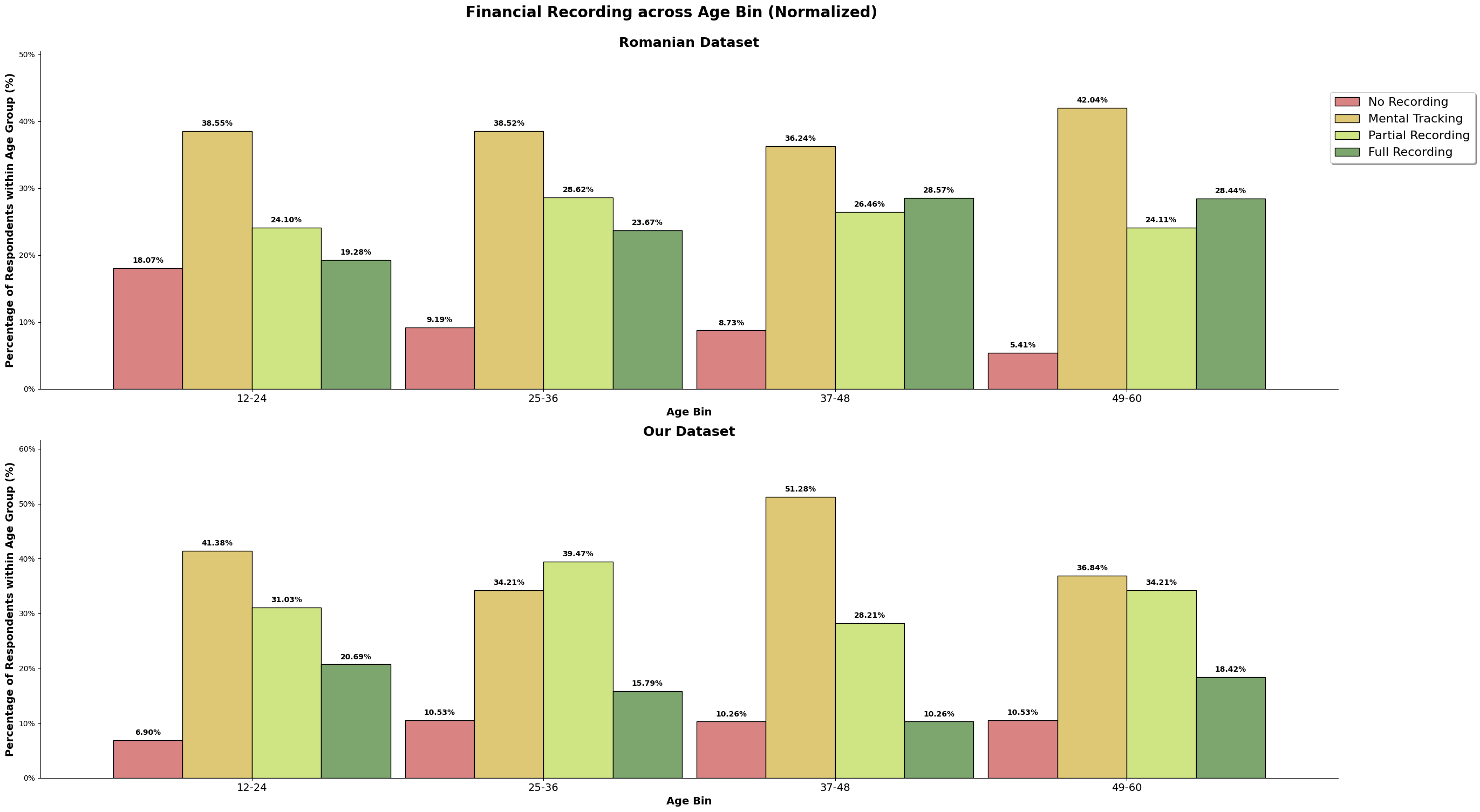
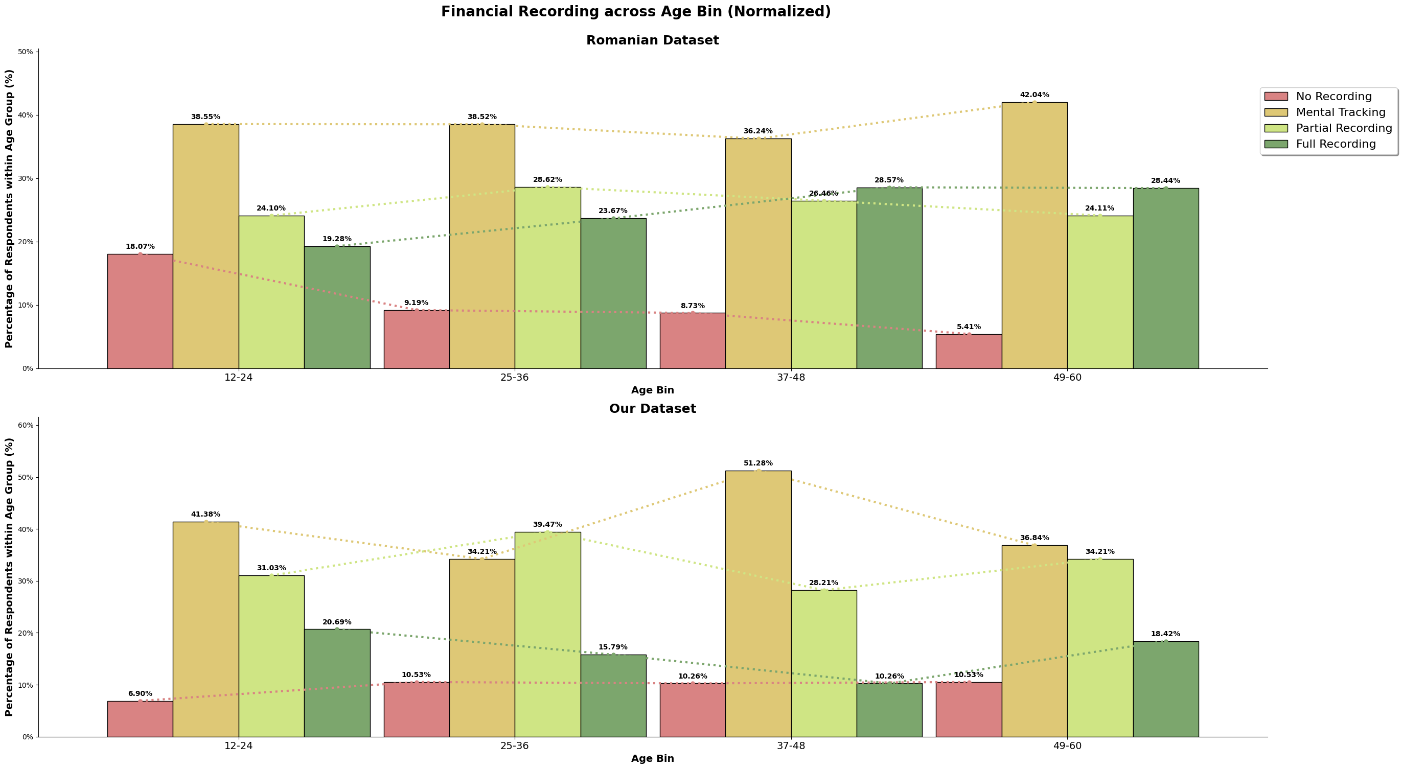
The two graphs shows the financial behaviour of recording/tracking one's financials for both datasets. Based on the romanian dataset, we do see that as the age increase, we see a decrease in those who has 'No Recording' and an increase of 'Full Recording'. 'Partial Recording' and 'Mental Recording' hovers around the same amount. This supports the claim that financial behaviour does increase with age.
For our dataset, the youngest age group had the lowest number of 'No Recording', with also the higest of 'Full Recording'. There are no definitive identifiable trend, unlike the romanian dataset. The only theory that we have is that after practicing 'Full Recording' at a younger age, we might slowly shift to 'Partial Recording' and 'Mental Tracking', as we might be able to estimate our income and spendings without effortful recording. Hence, we see an increase in 'Mental Tracking'. Then, in the final age group, where there is an increase in 'Partial Recording' and 'Full Recording' again, could be due to increase number of responsibilities and financial worry for the future.
Financial Behaviour and Gender - Does Gender affect Financial Behaviour?
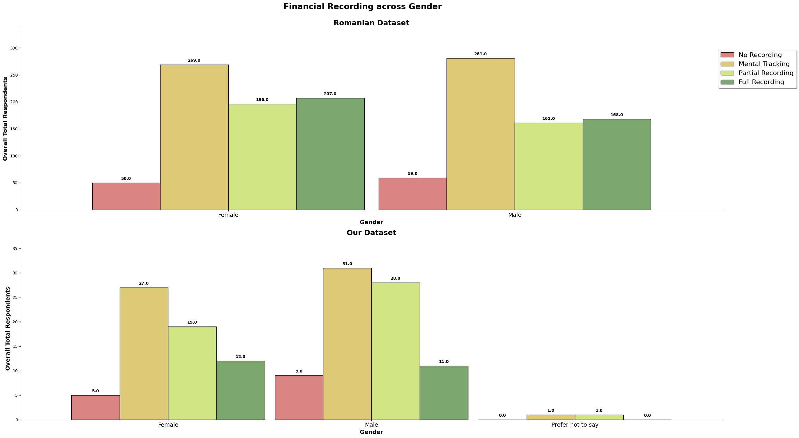
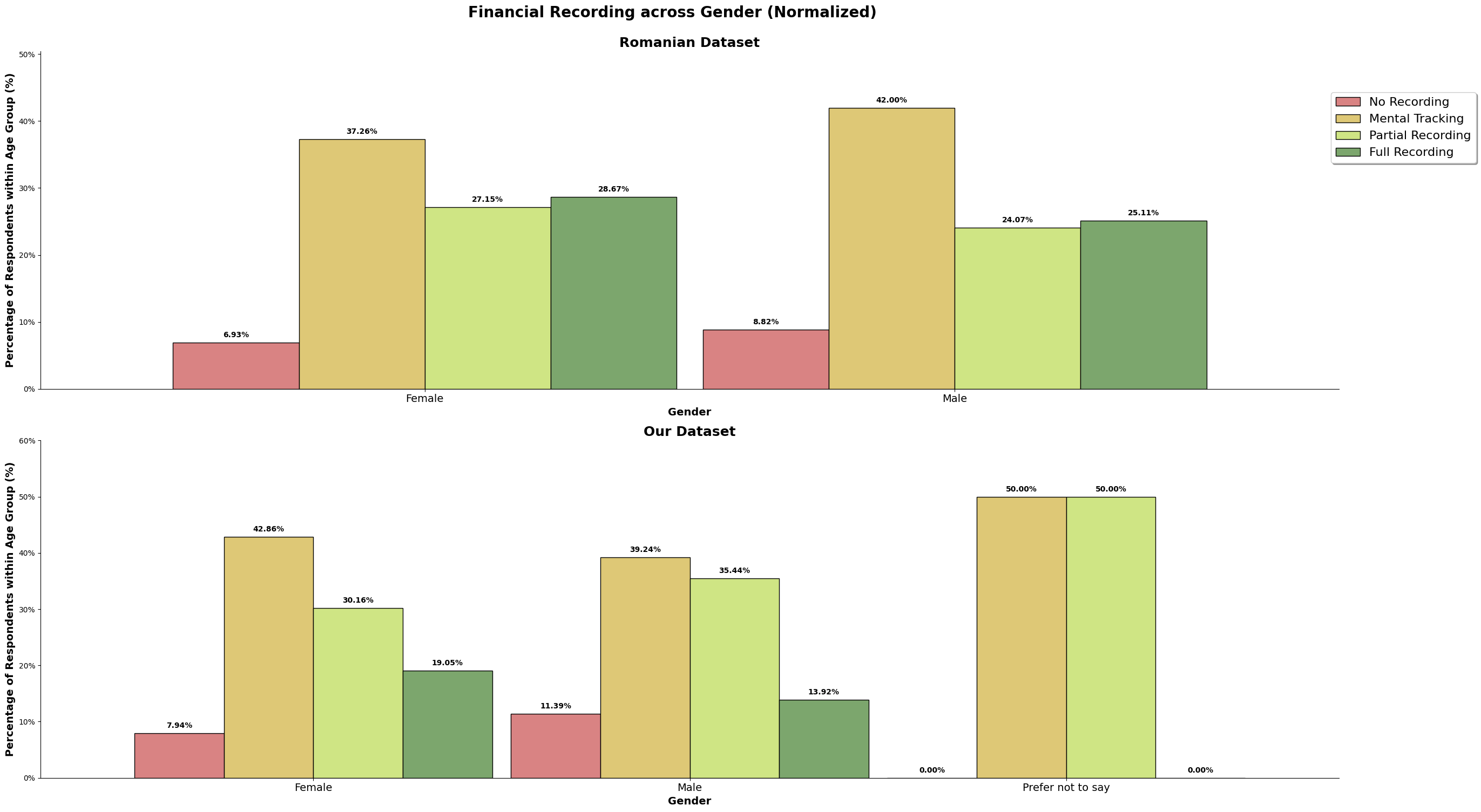
The difference between the normalized graph with the one not normalized, have little to no visible difference.
For the romanian dataset, we are able to observe that 'Female' seem to have a slight edge over 'Male', where 'Female' have ever so slightly lesser 'No Recordings' and 'Mental Tracking', and have slightly more 'Partial Recording' and 'Full Recording'.
As for our dataset, it is about equal, as we do see more 'No Recording' for 'Male' but 'Female' has higher 'Mental Tracking'. There is more 'Partial Recording' for "Male' but higher 'Full Recording' for 'Female'.
In the romanian dataset, Females have slight edge over Males, but based on our datset, the difference is not significant.
Financial Behaviour across Income Range - Do high-earners have better financial behaviour?

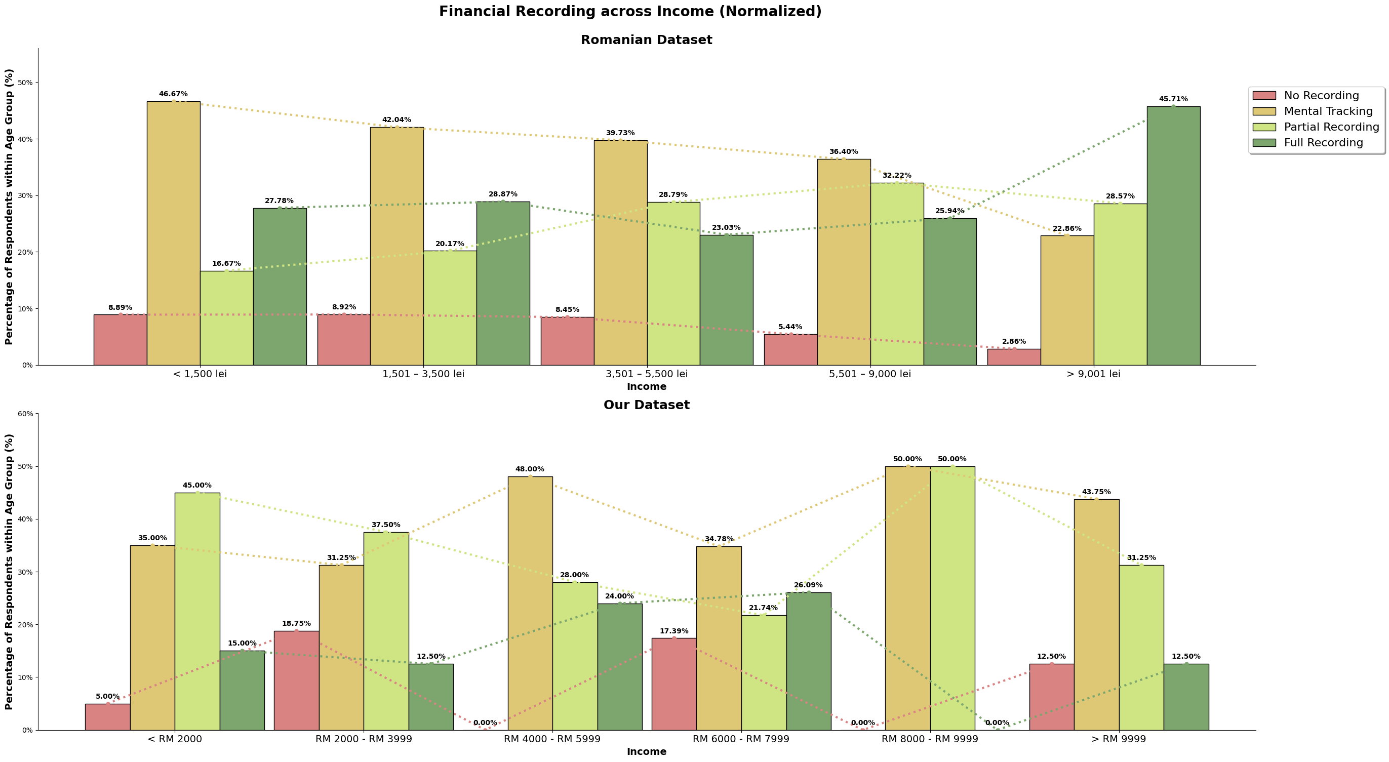
Using the graph with trend lines, we can clearly see, for the romanian dataset that desirable financial behaviour increase as income increases. We can see clear decreases for both 'No Recording' and 'Mental Tracking', and increases for 'Partial Recording' and 'Full Recording'.
For our dataset, we do not see any clear trends to support any claims. Excluding the last two income groups, we do see a decreasing trend in 'Partial Recording', but an increase 'Full Recording'. However, that does not tell us much.
Financial Behaviour across Education Attaiment - Does education equate to better behaviour?

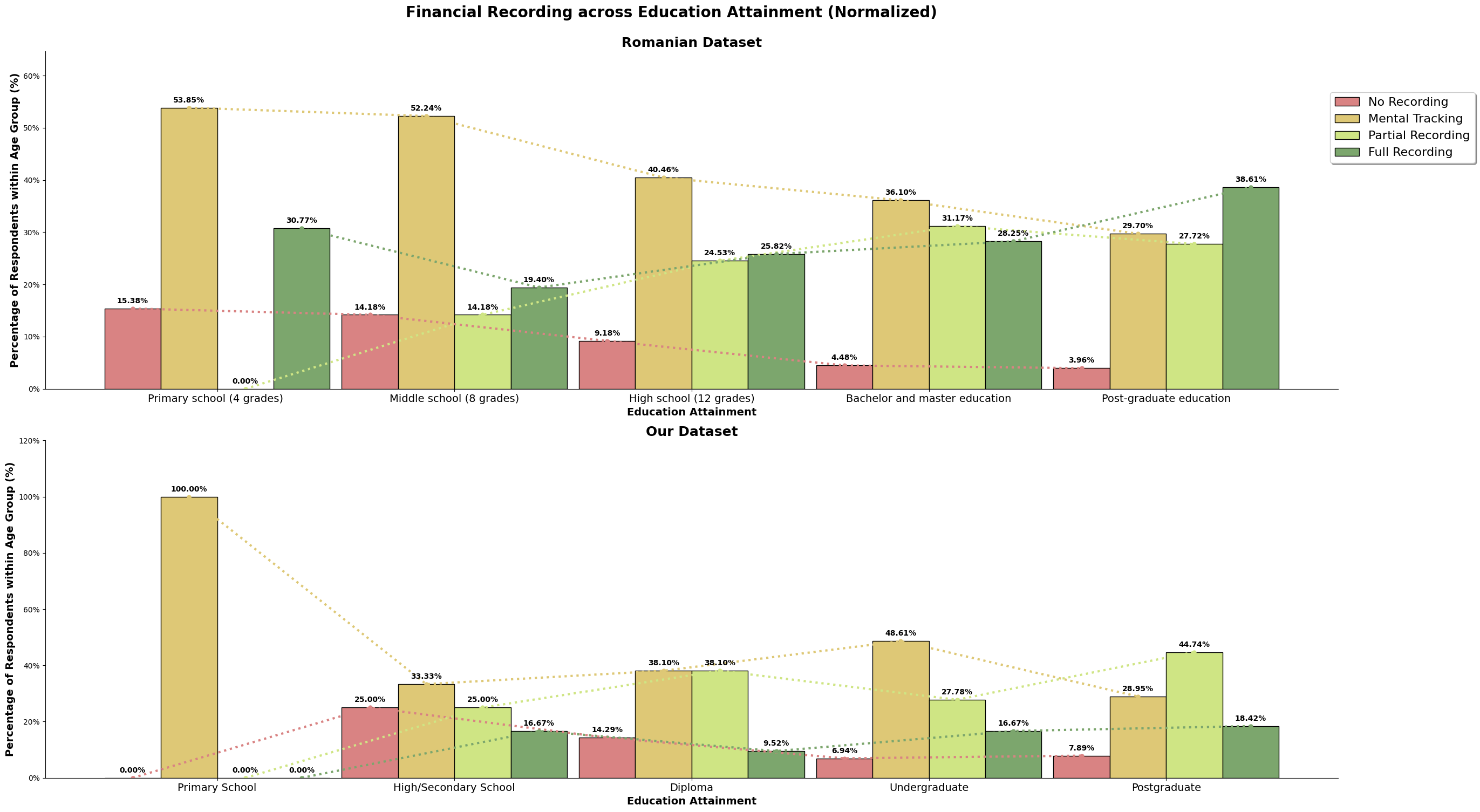
The above graph shows the normalized values of financial behaviour across eduaction attainment for both datasets.
We can see that for the romanian dataset again, has a clear trend of having higher education attainment, translate to better financial behaviour. For both the 'No Recording' and 'Mental Tracking', we see a trending decrease, while for the 'Partial Recording' and 'Full Recording', we see an increase as the education attainment increases as well.
For our dataset, only the 'No Recording' has a clear decreasing trend, which at least support the fact that having a higher education attainment, causes some form recording to be perform.
def create_financial_recording_graph(our_column, romanian_column, title:str, normalize:bool=False, lineplot:bool=False,
                        our_dataset=our_dataset, romanian_dataset=romanian_dataset):

    # Data Preparation
    # =================
    romanian_df = romanian_dataset[[romanian_column, 'Financial Recording']].groupby(romanian_column, observed=False)\
        .value_counts(normalize=normalize)

    our_df = our_dataset[[our_column, 'Financial Recording']].groupby(our_column, observed=False)\
        .value_counts(normalize=normalize)

    # Plot Figure
    # ============
    # Initialize Figure
    fig, (ax1, ax2) = plt.subplots(2, 1, figsize=(25,15) )
    fig.suptitle(f'Financial Recording across {title}' + (' (Normalized)' if normalize else ''),
                 fontweight='bold', size=20, y=1)

    # Set color lists
    color_set = ["#D98383", "#DEC876", "#CFE584", "#7CA66D"]

    formatter = mtick.PercentFormatter(xmax=1.0, decimals=None)

    # Set values to loop
    datasets = [
        (romanian_df, 'Romanian Dataset', ax1),
        (our_df, 'Our Dataset', ax2)
    ]

    # Looping through the values
    for dataset, subtitle, ax in datasets:

        df_plot = dataset.unstack()
        width = 0.95

        # Plot bar
        df_plot.plot(kind='bar', ax=ax, color=color_set, edgecolor='black', width=width, rot=0)

        if normalize and lineplot:
            # Calculate coordinates for the lines
            n_groups = len(df_plot)
            n_bars_per_group = len(df_plot.columns)
            individual_bar_width = width / n_bars_per_group

            # Plot lines using calculated X offsets
            for i, col_name in enumerate(df_plot.columns):

                # Calculate the horizontal shift for the i-th bar in the group
                offset = (i - (n_bars_per_group - 1)/2) * individual_bar_width
                x_positions = [p + offset for p in range(n_groups)]

                ax.plot(x_positions, df_plot[col_name],
                        color=color_set[i],
                        marker='o', markersize=5,
                        label='_nolegend_',
                        linestyle=':', linewidth=3)

        # Bar labels and formatting
        for c in ax.containers:
            ax.bar_label(c, fmt='{:.2%}' if normalize else '{:}', fontweight='bold', fontsize=10, padding=5)

        ax.set_title(subtitle, fontsize=18, fontweight='bold')

        if normalize:
                ax.yaxis.set_major_formatter(formatter)
                ax.set_ylabel('Percentage of Respondents within Age Group (%)', fontweight='bold', fontsize=14)
        else:
            ax.set_ylabel('Overall Total Respondents', fontweight='bold', fontsize=14)

        ax.set_xlabel(f'{title}', fontweight='bold', fontsize=14)
        ax.legend().remove()
        ax.spines[['top', 'right']].set_visible(False)
        ax.tick_params(axis='x', labelsize=14)
        ax.set_ylim(0,max(dataset)*1.2)

    fig.legend(financial_recording_label, fontsize=16, shadow=True, bbox_to_anchor=(1.1,0.9))
    plt.tight_layout()
    plt.show()

# Financial Recording / Behaviour across Age Bin
create_financial_recording_graph('Age Bin', 'Age Bin', 'Age Bin', False)
create_financial_recording_graph('Age Bin', 'Age Bin', 'Age Bin', True)
create_financial_recording_graph('Age Bin', 'Age Bin', 'Age Bin', True, True)

# Financial Recording / Behaviour across Genders
create_financial_recording_graph(our_gender_string, romanian_gender_string, 'Gender', False)
create_financial_recording_graph(our_gender_string, romanian_gender_string, 'Gender', True)

# Financial Recording / Behaviour across Income Range
create_financial_recording_graph(our_income_string, romanian_income_string, 'Income', False)
create_financial_recording_graph(our_income_string, romanian_income_string, 'Income', True)
create_financial_recording_graph(our_income_string, romanian_income_string, 'Income', True, True)

# Financial Recording / Behaviour across Education Attainment
create_financial_recording_graph(our_education_string, romanian_education_string, 'Education Attainment', False)
create_financial_recording_graph(our_education_string, romanian_education_string, 'Education Attainment', True)
create_financial_recording_graph(our_education_string, romanian_education_string, 'Education Attainment', True, True)
Financial Literacy based on other factors
Financial Literacy across Genders - Who is money-smarter?
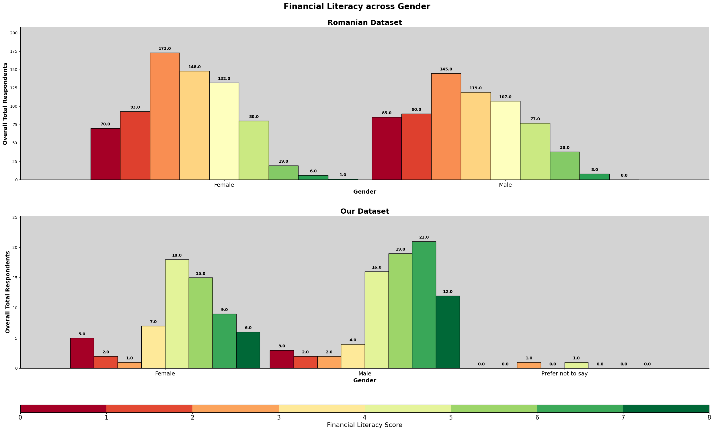
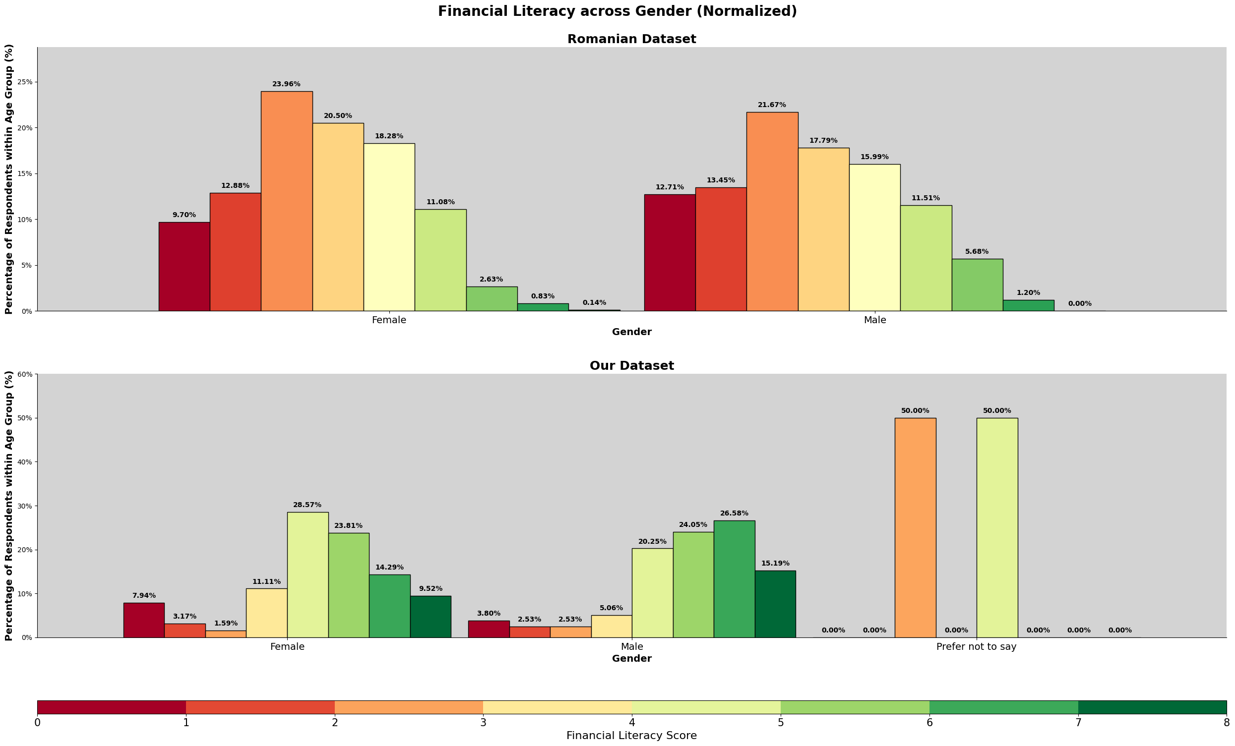
In the romanian dataset, we can see that Males has a slightly higher percentage over female in score 6 and 7. However, Males have higher percentage of lower scores as well, in 0 and 1. Females scored higher in the middle range score of 2, 3 and 4.
For our dataset, we once again, do see that there are higher percentage of Males in the higher range of scores, while Females have higher percentage in the middle range of the scores.
The romanian dataset shows equality of financial literacy among males and females, but our dataset does not.
Financial Literacy across Income - Does being money-smart make you more money?
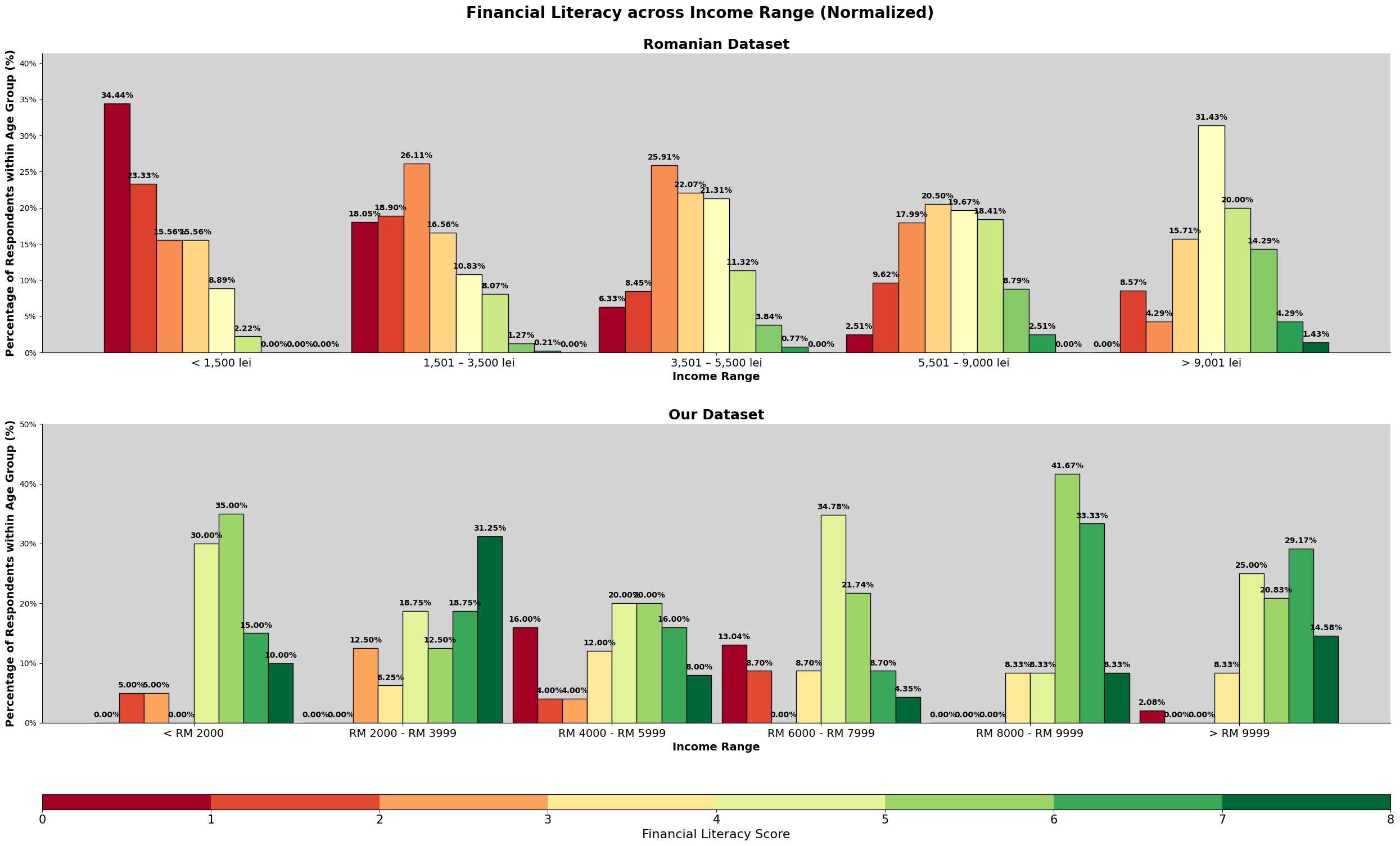
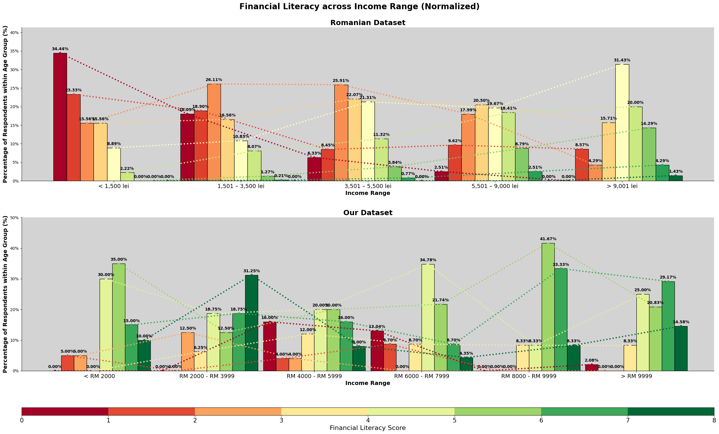
Both the graphs are normalized values are financial literacy across income range for both datasets.
We can observed in the romanian dataset that the lower range of financial literacy scores, does decrease as income increases. We can also see the opposite where the higher range of financial literacy score increases as income increases. Hence, the claim that having higher financial literacy increases income, is supported.
However, for our dataset, we do not see any paticular trends that can support the claim. We do notice that financial literacy is high throughout the income range, but it is the highest at income range 'RM2000 - RM3999'.
Financial Literacy across Age Groups - Does being older equate to higher financial literacy?
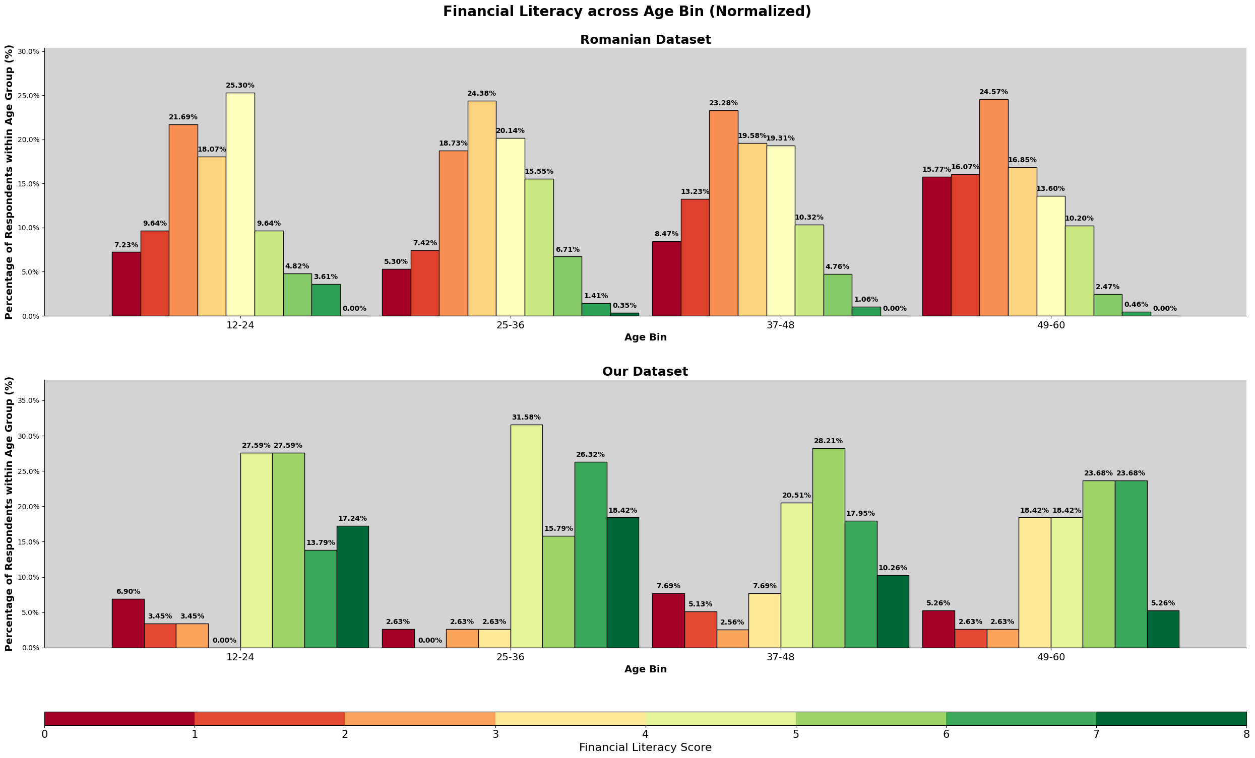
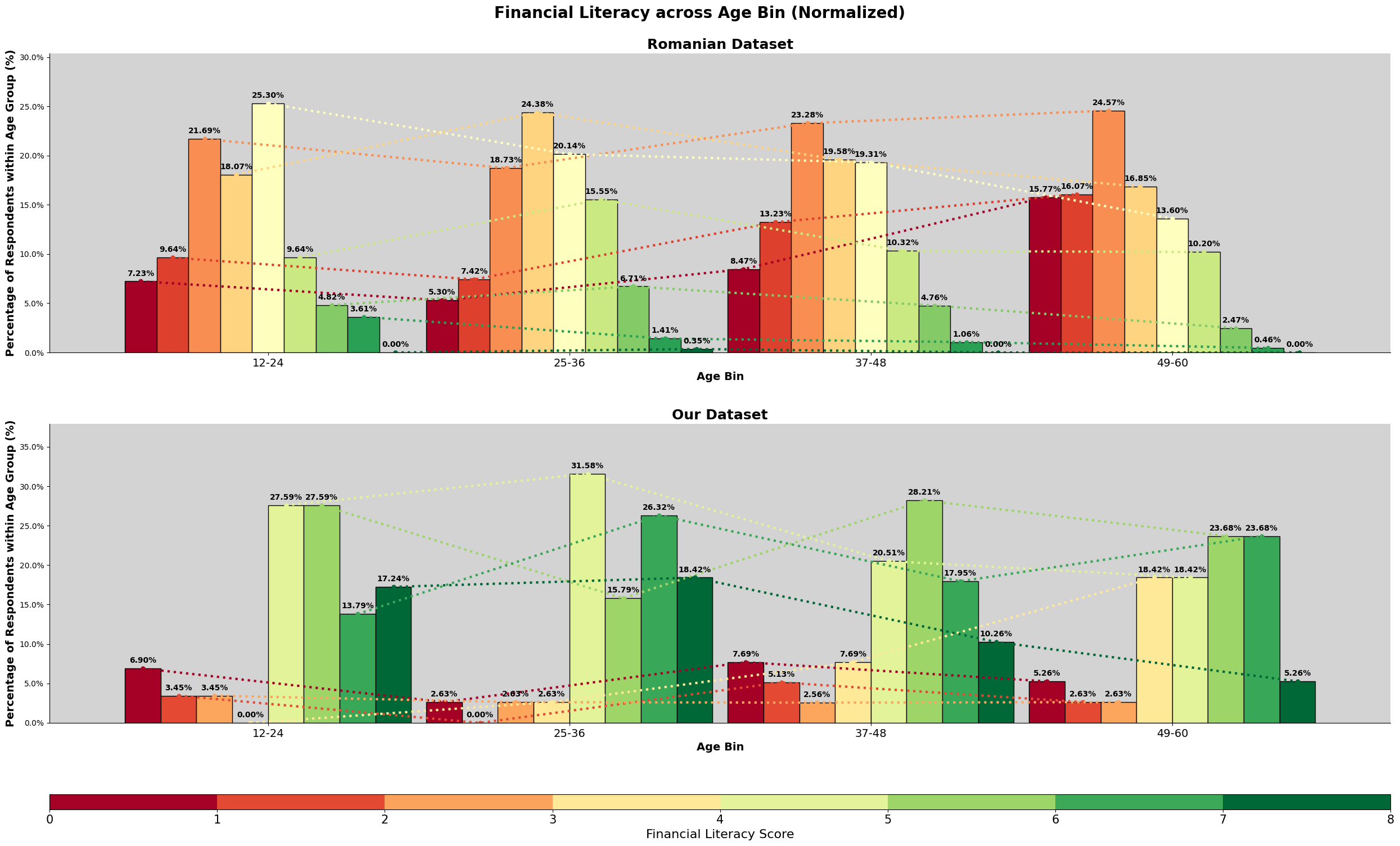
These graph show the normalized values of financial literacy across age gropus for both datasets.
One would expect the older we get, the better understanding of financial literacy one would have. However, both romanian dataset and our dataset shows the contrary. In the romanian dataset, we see a rise in the lower range scores and decline in the higher range scores as we move along the age groups. For our dataset, we see a decrease of higher range score the further the age group. This might be because the awareness and importance of financial literacy being emphasized to the younger generations.
Financial Literacy across Education Attainment - Does being smart mean you are financially smart too?
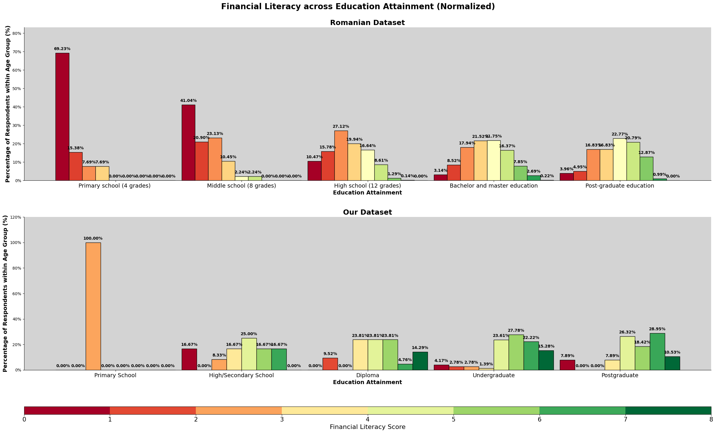

The graphs shows the normalized values for financial literacy across education attainment for both datasets.
We can observe that an definite trend in the romanian dataset where the lower range of financial literacy drops the higher the education attainent.
For our dataset, we do also see that education attainment play a role in financial literacy, as we can see the lower range of the score decrease.
def create_financial_literacy_graph(our_column, romanian_column, title:str,
                                    normalize:bool=False, lineplot:bool=False,
                                    our_dataset=our_dataset, romanian_dataset=romanian_dataset):

    # Data Preparation
    # =================
    romanian_df = romanian_dataset[[romanian_column, 'Financial Literacy Score']]\
        .groupby(romanian_column, observed=False).value_counts(normalize=normalize)

    our_df = our_dataset[[our_column, 'Financial Literacy Score']]\
        .groupby(our_column, observed=False).value_counts(normalize=normalize)

    # Plot Figure
    # ============
    fig, (ax1, ax2, ax3) = plt.subplots(3, 1, figsize=(25,15), gridspec_kw={'height_ratios': [20,20,1]},  )
    fig.suptitle(f'Financial Literacy across {title}' + (' (Normalized)' if normalize else ''),
                 fontweight='bold', size=20, y=1)

    ax1.set_facecolor('lightgrey')
    ax2.set_facecolor('lightgrey')

    # Set values to loop
    datasets = [
        (romanian_df, 'Romanian Dataset', ax1),
        (our_df, 'Our Dataset', ax2)
    ]

    formatter = mtick.PercentFormatter(xmax=1.0)

    # Set colorbar
    colorbar_cmap = mpl.cm.RdYlGn
    financial_literacy_bounds = [x for x in range(9)]
    norm = mpl.colors.BoundaryNorm(financial_literacy_bounds, colorbar_cmap.N)
    fig.colorbar(mpl.cm.ScalarMappable(norm=norm, cmap=colorbar_cmap),
                 cax=ax3, orientation='horizontal')
    ax3.set_xlabel('Financial Literacy Score', fontsize=16)
    ax3.tick_params(axis='x', labelsize=15)

    # Looping through the values
    for dataset, subtitle, ax in datasets:

        df_plot = dataset.unstack()
        width = 0.95

        # Plot bar
        df_plot.plot(kind='bar', ax=ax, cmap='RdYlGn', edgecolor='black', width=width, rot=0)

        if normalize and lineplot:
            # Calculate coordinates for the lines
            n_groups = len(df_plot)               # Number of Age Bins
            n_bars_per_group = len(df_plot.columns) # Number of Literacy Scores
            individual_bar_width = width / n_bars_per_group

            # Get the colormap to match line colors to bar colors
            color_set = [mpl.cm.RdYlGn(i / (n_bars_per_group - 1)) for i in range(n_bars_per_group)]

            # Plot lines using calculated X offsets
            for i, col_name in enumerate(df_plot.columns):

                # Calculate the horizontal shift for the i-th bar in the group
                offset = (i - (n_bars_per_group - 1)/2) * individual_bar_width
                x_positions = [p + offset for p in range(n_groups)]

                ax.plot(x_positions, df_plot[col_name],
                        color=color_set[i],
                        marker='o', markersize=5,
                        label='_nolegend_',
                        linestyle=':', linewidth=3)

        # Bar labels and formatting
        for c in ax.containers:
            ax.bar_label(c, fmt='{:.2%}' if normalize else '{:}', fontweight='bold', fontsize=10, padding=5)

        ax.set_title(subtitle, fontsize=18, fontweight='bold')

        if normalize:
            ax.yaxis.set_major_formatter(formatter)
            ax.set_ylabel('Percentage of Respondents within Age Group (%)', fontweight='bold', fontsize=14)
        else:
            ax.set_ylabel('Overall Total Respondents', fontweight='bold', fontsize=14)

        ax.set_xlabel(f'{title}', fontweight='bold', fontsize=14)
        ax.spines[['top', 'right']].set_visible(False)
        ax.tick_params(axis='x', labelsize=14)
        ax.legend().remove()
        ax.set_ylim(0,max(dataset)*1.2)

    plt.tight_layout()
    plt.subplots_adjust(hspace=0.35)
    plt.show()

# Financial Literacy by Gender
create_financial_literacy_graph(our_gender_string, romanian_gender_string, 'Gender', False)
create_financial_literacy_graph(our_gender_string, romanian_gender_string, 'Gender', True)

# Financial Literacy across Income Range
create_financial_literacy_graph(our_income_string, romanian_income_string, 'Income Range', False)
create_financial_literacy_graph(our_income_string, romanian_income_string, 'Income Range', True)
create_financial_literacy_graph(our_income_string, romanian_income_string, 'Income Range', True, True)

# Financial Literacy by Age Bin
age_bin_string = 'Age Bin'
create_financial_literacy_graph(age_bin_string, age_bin_string, age_bin_string, False)
create_financial_literacy_graph(age_bin_string, age_bin_string, age_bin_string, True)
create_financial_literacy_graph(age_bin_string, age_bin_string, age_bin_string, True, True)

# Financial Literacy across Education Attainment
create_financial_literacy_graph(our_education_string, romanian_education_string, 'Education Attainment')
create_financial_literacy_graph(our_education_string, romanian_education_string, 'Education Attainment', True)
create_financial_literacy_graph(our_education_string, romanian_education_string, 'Education Attainment', True, True)
Financial Well-Being based on other factors
Financial Well-Being across Age Group - Does being older mean more financial stability?
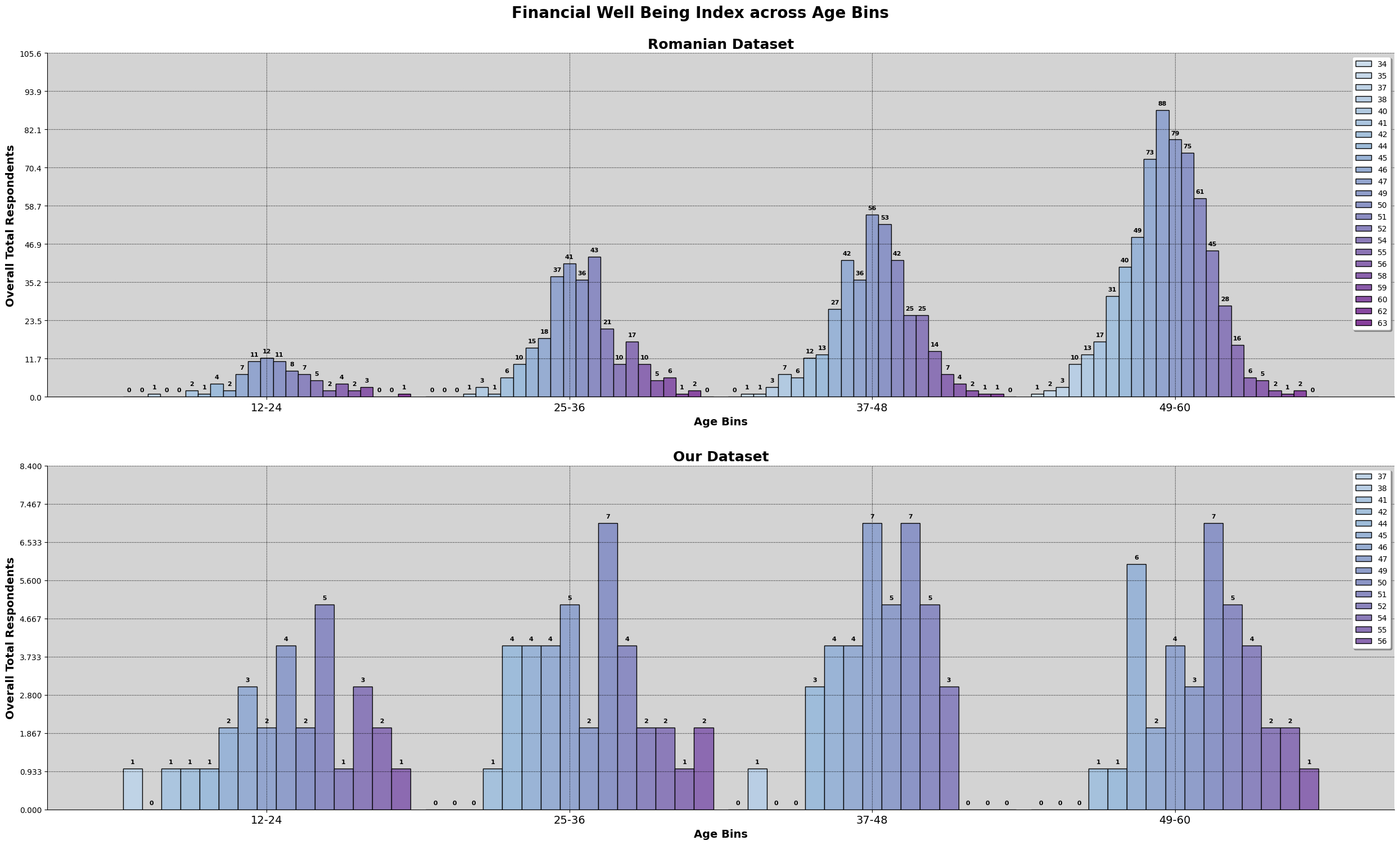
This graph shows the financial well being score across the age group, not normalized. We can see that in each age group for both dataset, exist a range of financial well being statuses regardless of age.
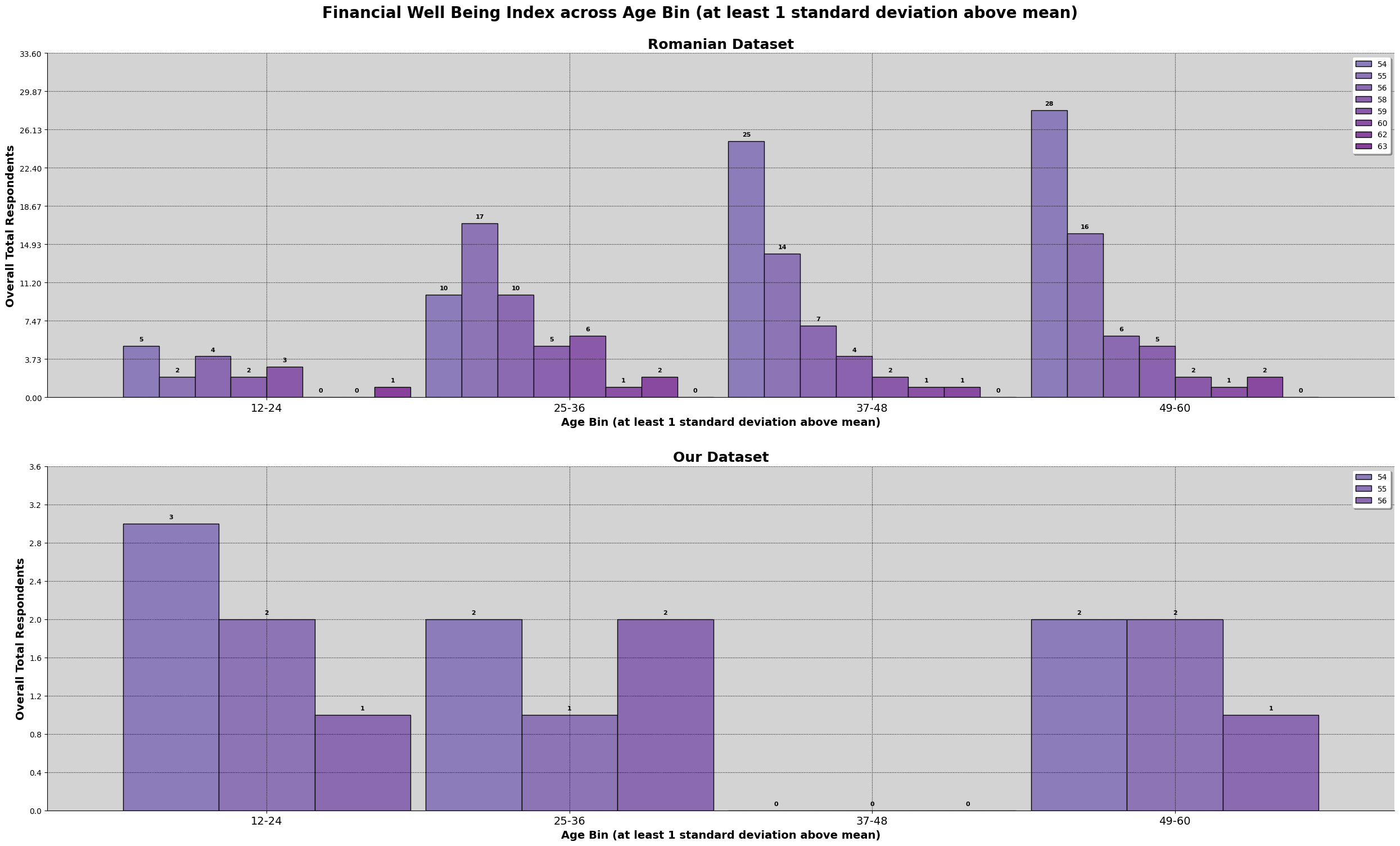
This graph is filtered, for those that have financial well being of above one standard deviation above the mean. In our dataset, we do see the 37-48 age group not having any, but we believe it is due to the insufficient data. The raising for the romanian dataset is due to its distribution shape of the dataset, as shown in this section.
Financial Well-Being across Genders - Is it financially happier to be a Girl or Guy?
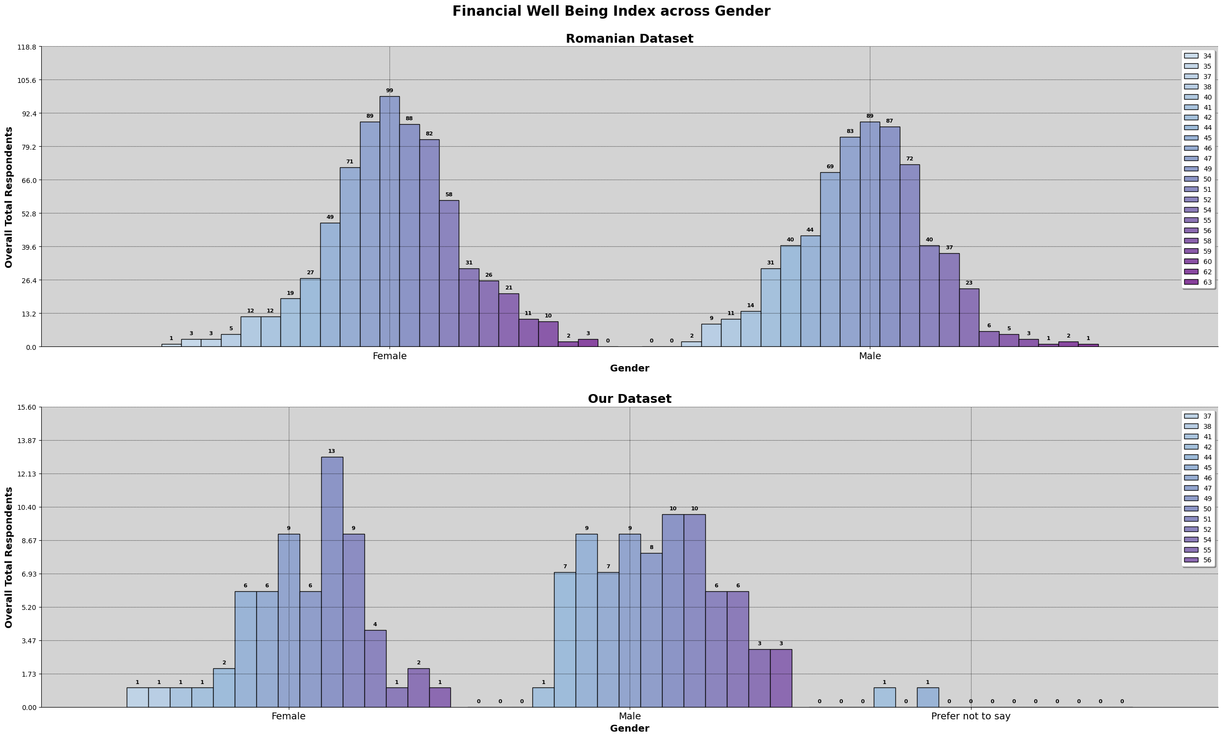
Similar to above sections when comparing genders, it seems that for the romanian dataset, the difference between male and female are indistinguishable. As for our dataset, while there seem to be a bit more male on the higher range of financial well being range, but it could also be not having sufficient data collect by us.
Hence, gender does not affect the financial well being of an individual.
Financial Well-Being across Income Range - More money more happy?
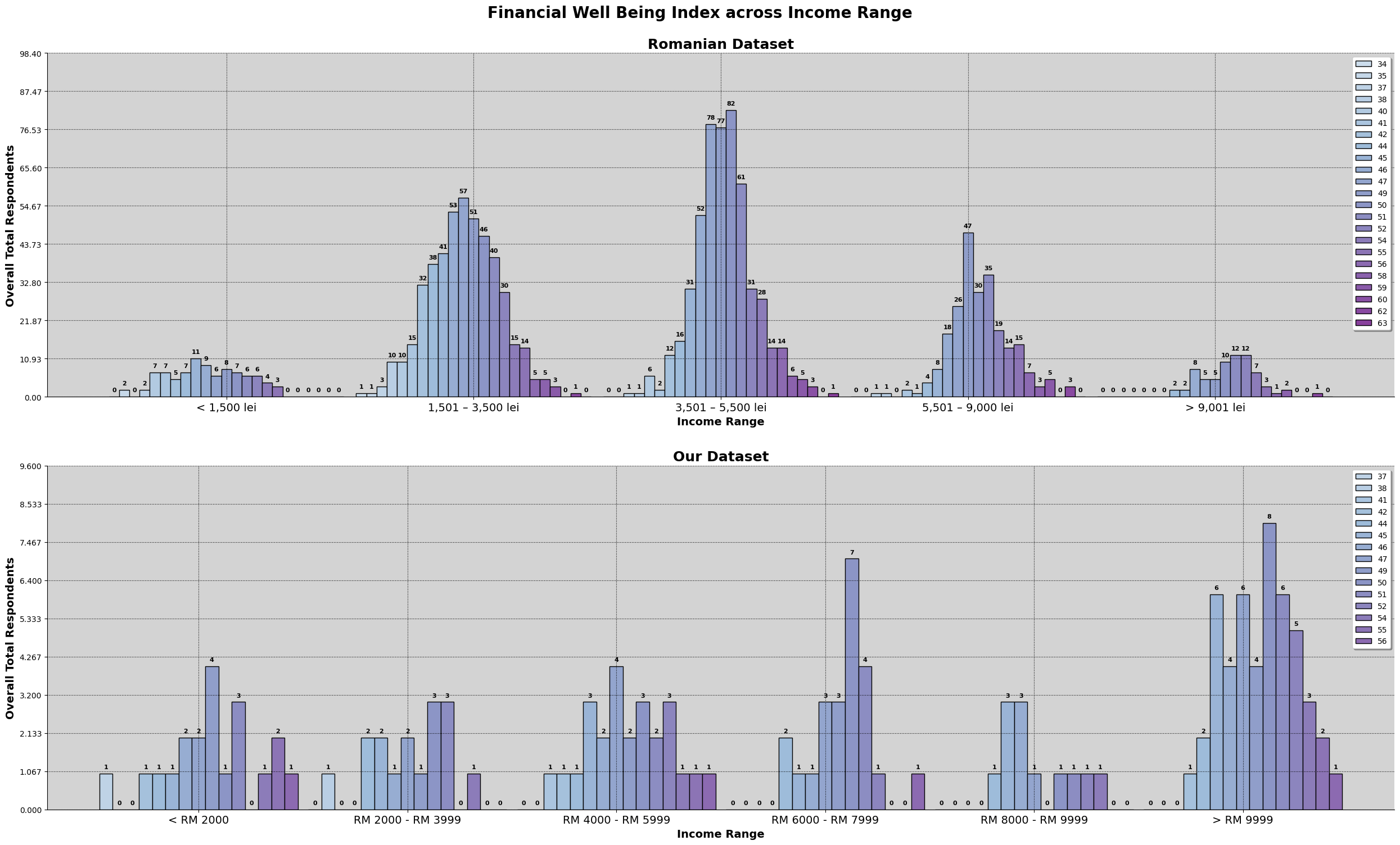
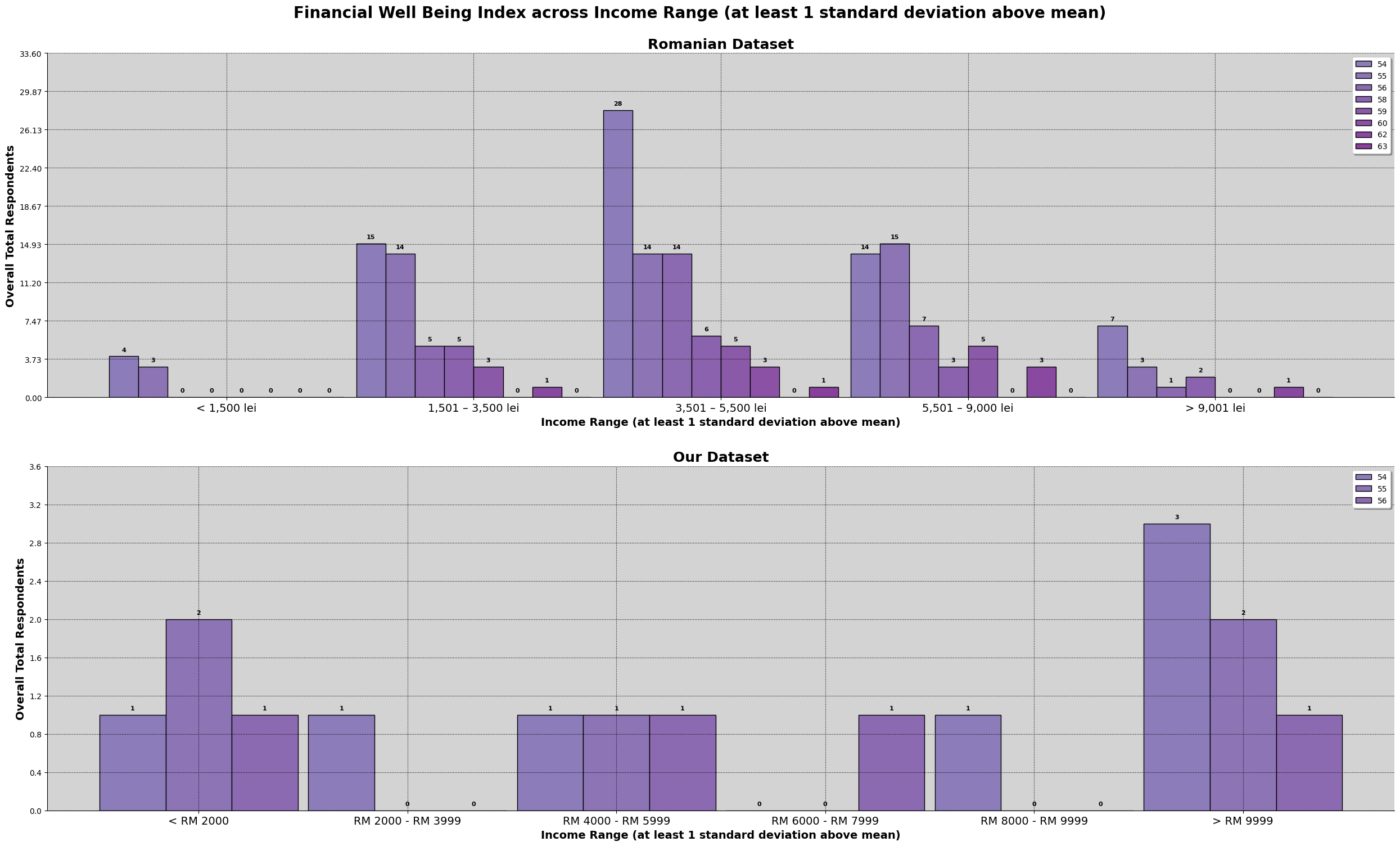
The top graph is the financial well being score across income ranges, not normalized for both dataset, and the bottom graph is the same, but filtered for those that are above financial well being mean by one standard deviation and above.
We also see that financial well being above the mean, do exist regardless of income range. Visually, we cannot really conclude any relationship.
Financial Well-Being across Education Attainment - Does being smart mean being happy?
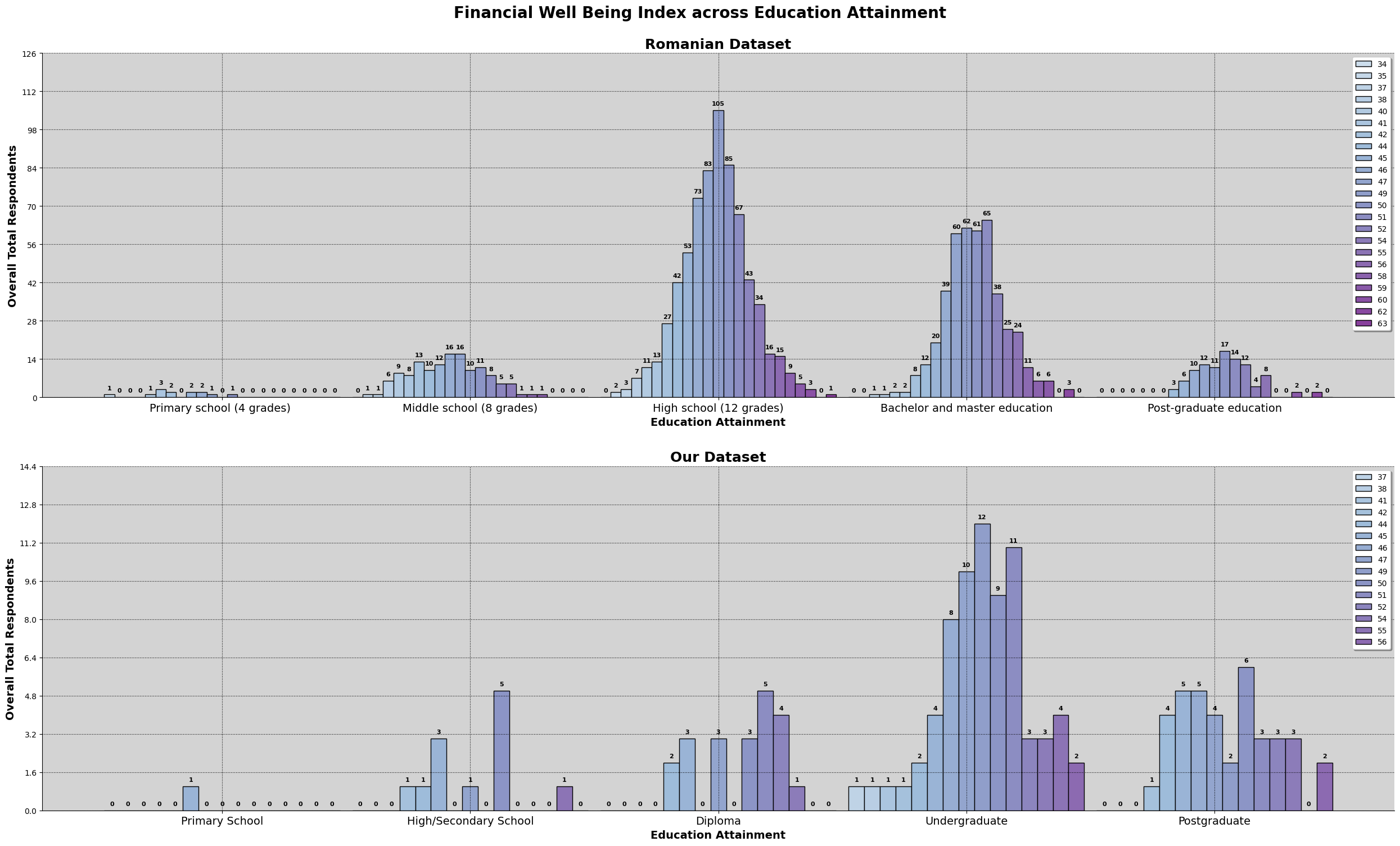
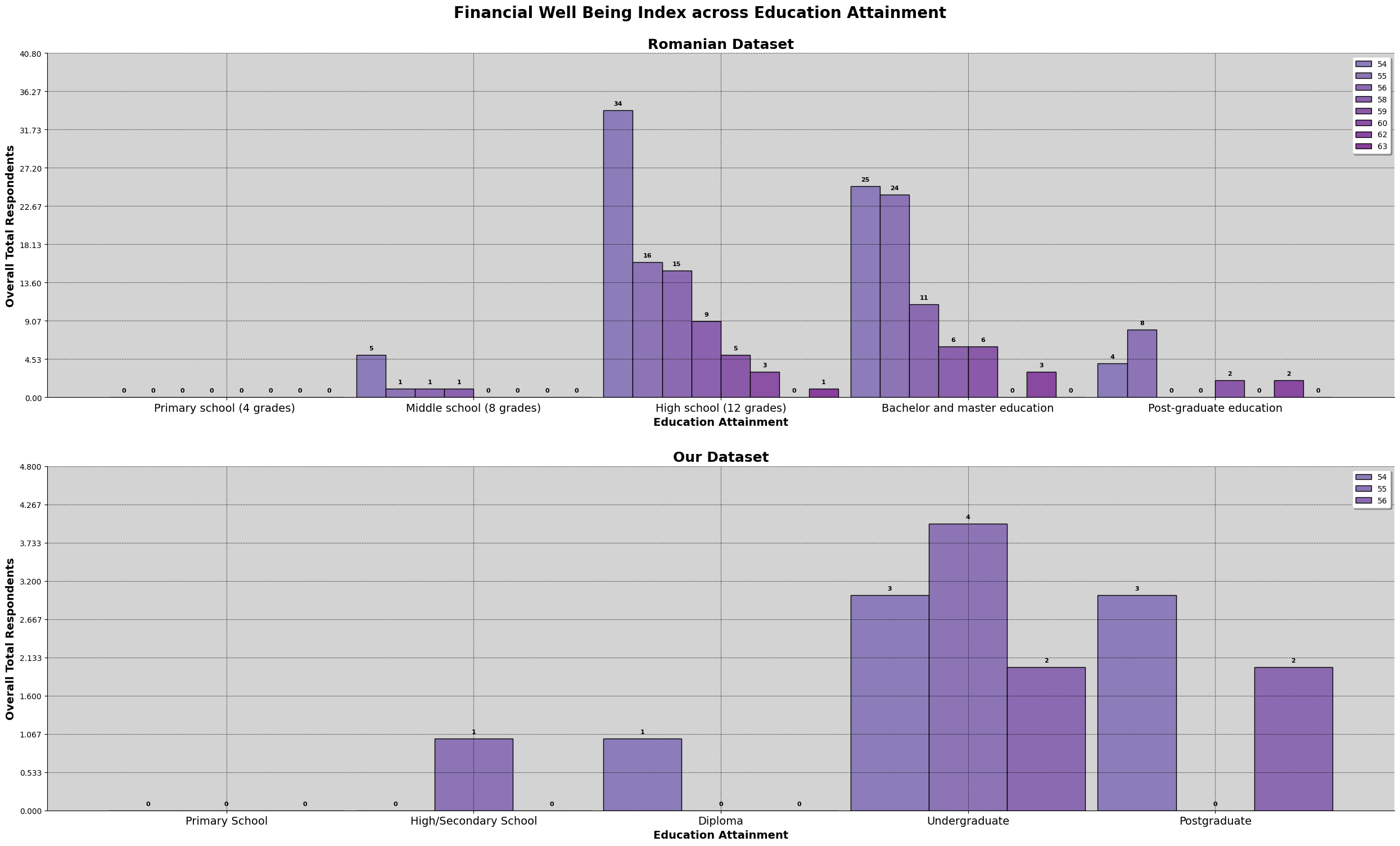
The top graph is the financial well being score across education attainment, not normalized for both dataset, and the bottom graph is the same, but filtered for those that are above financial well being mean by one standard deviation and above.
We also do see financial well being range across all education attainment. Visually, we cannot conclude any relationship.
Financial Well-Being and Financial Literacy - Does being money-smart bring financial bliss?
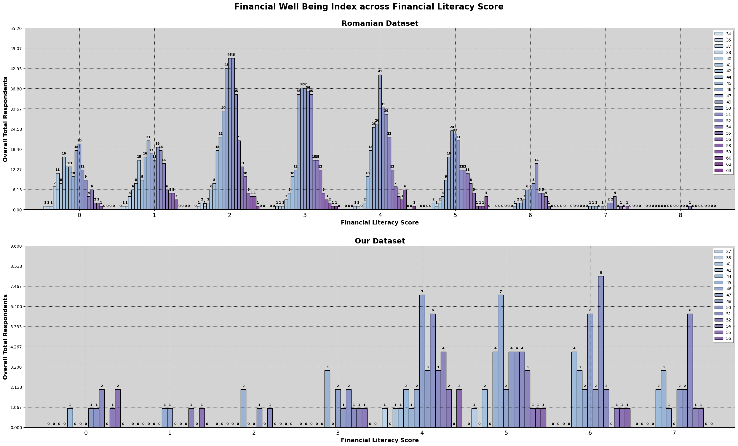
This graph shows the financial well being index across financial literacy score. At a glance we also see that financial well being range exist regardless of financial literacy score.
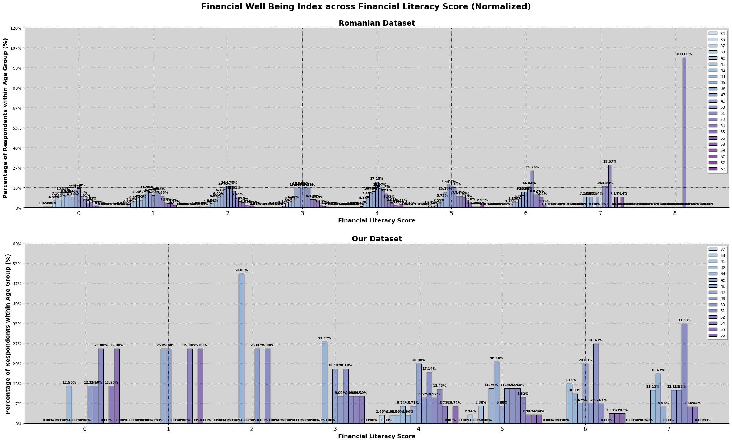
Even with the normalized graph, we see that it exists in a range, regardless of financial literacy.
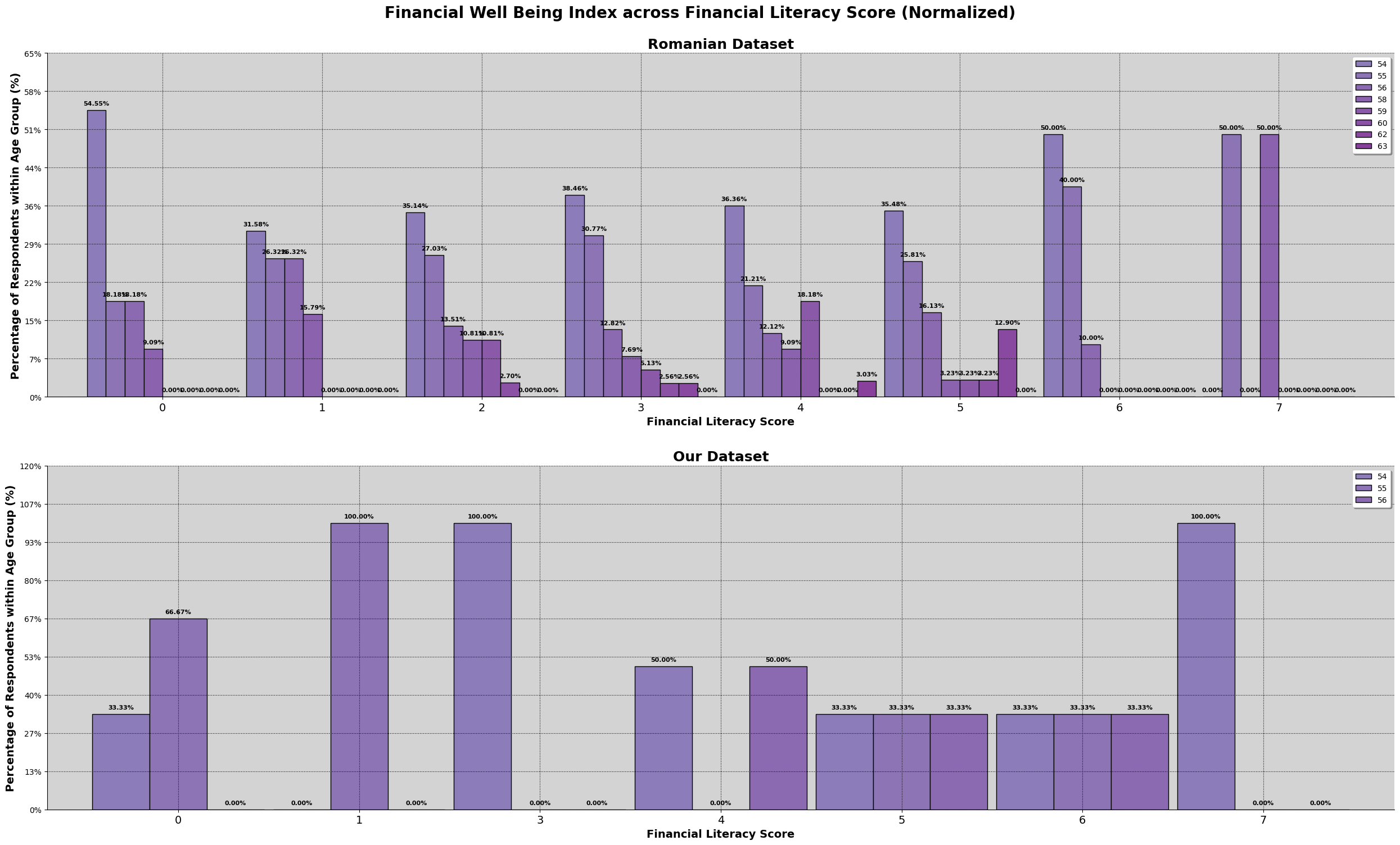
Even after filtering, we still see that above average financial well being, exists even if financial literacy score is on the lower end.
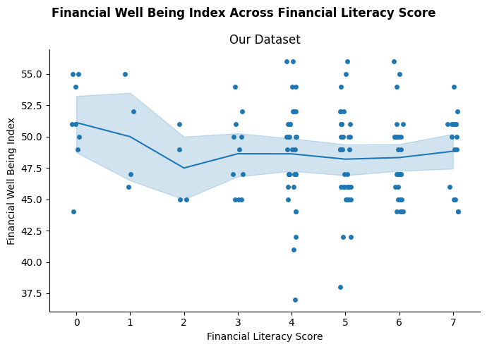
So we tried plotting it this way, to see if we can visually identify any patterns or relationships. For our dataset, we can observe relatively straight line across. That means regardless of financial literacy, there are individuals that have relatively high or low financial literacy score. It is even more boggling that financial literacy score of 4 and 5, has even lower lows then the other scores.
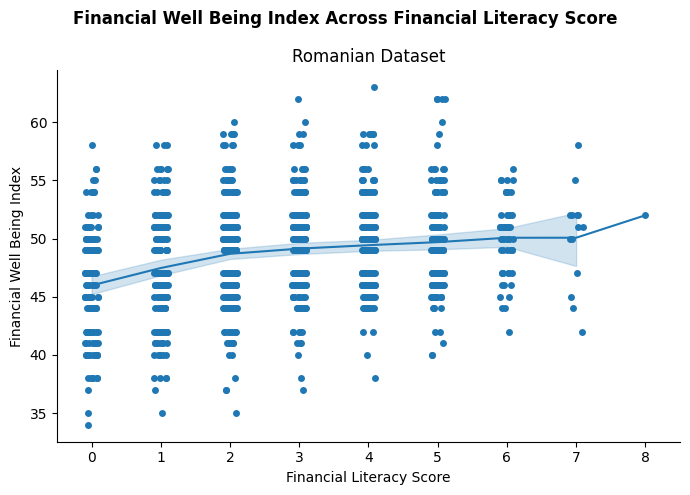
But for the romanian dataset, there is a slight trend that we can observe, it is still a relatively straight line across. However, we can see that with the increase of financial literacy score, the higher the lows and the highs. If we see the bottom and top of the strip plot, or the dotted points, we see an upward trend in the lowest points and highest points. Therefore, with the increase in financial literacy, the baseline of financial well being increases.
Financial Decision Influence - Deeper Dive
Based on the section above on Financial Decision Influence, we found that 'Social Media' and 'Advice from Family' were the highest two factors for influencing financial decisions, and 'Financial Advisor' was the lowest, so we thought to explore a little on these factors.
Social Media Influence over Age Group - Which generation rely more on Social Media?
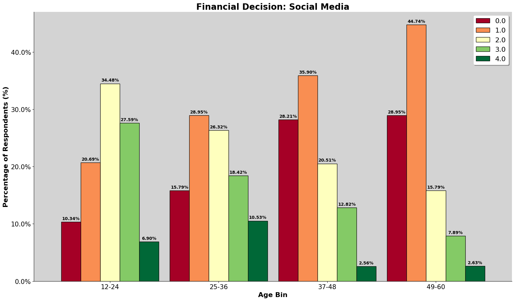

Based on the graphs, we can see that influence score of 0 and 1 increases as age group increases, and influence score of 2, 3, and 4 decreases as age increases. This shows that the younger generation rely on social media more than older generations for their financial decisions.
Social Media Influence over Education Attainment - Trust in education or Social Advice?
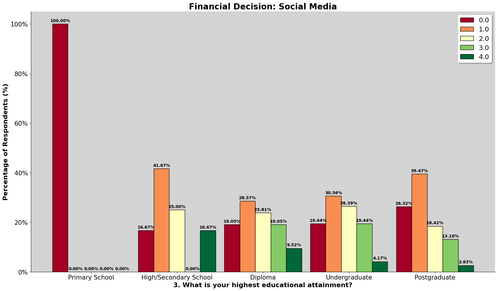
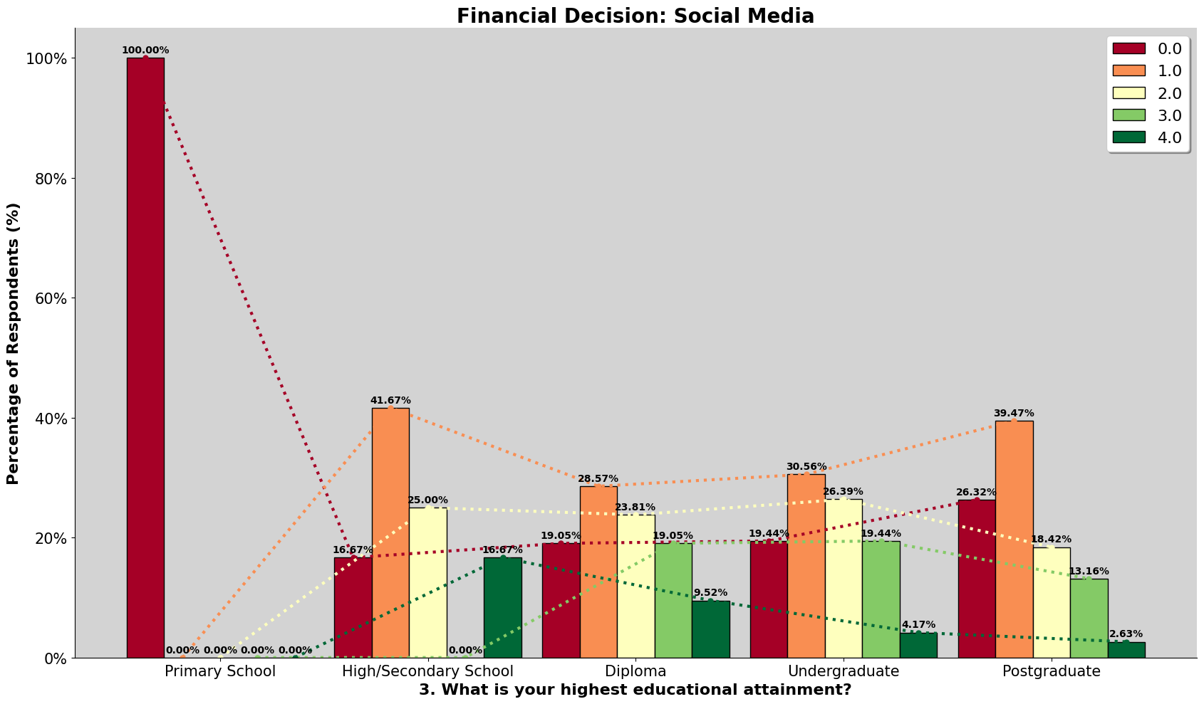
Based on the graphs, ignoring the 'Primary School' education attainment level, we can see that the score of 0 and 1 increases the higher the education attainment. The score of 2 remains about the same until a drop in 'Postgraduate', and we can see a clear decrease in score 4, as education attainment increases. Therefore, having higher education level, does make an individual rely less on social media for financial decisions.
Social Media Influence over Gender - Who believes in social media more?
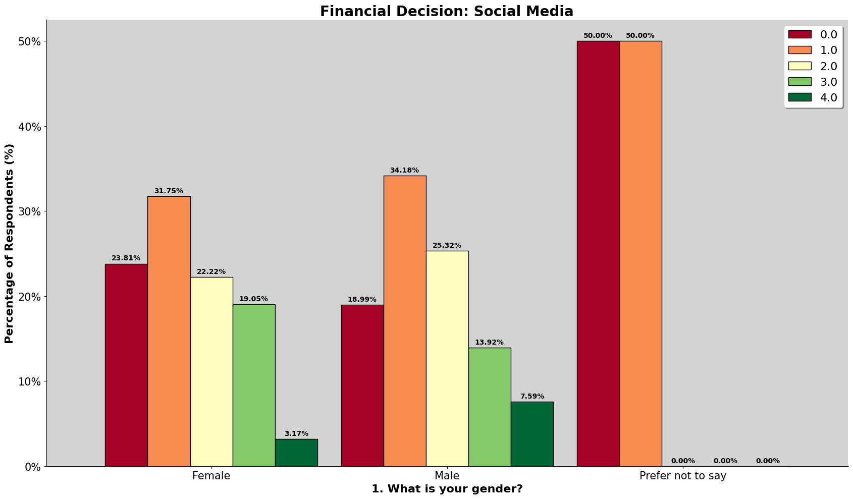
Based on the graph, the difference between male and female are not too different. While score 3 were higher with female than male, the score of 4 were higher in male than female. Therefore, social media influence over financial decisions are the same between genders.
Advice from Family over Age Groups - Do we still listen to our family?
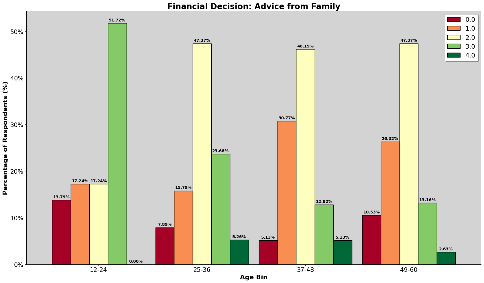
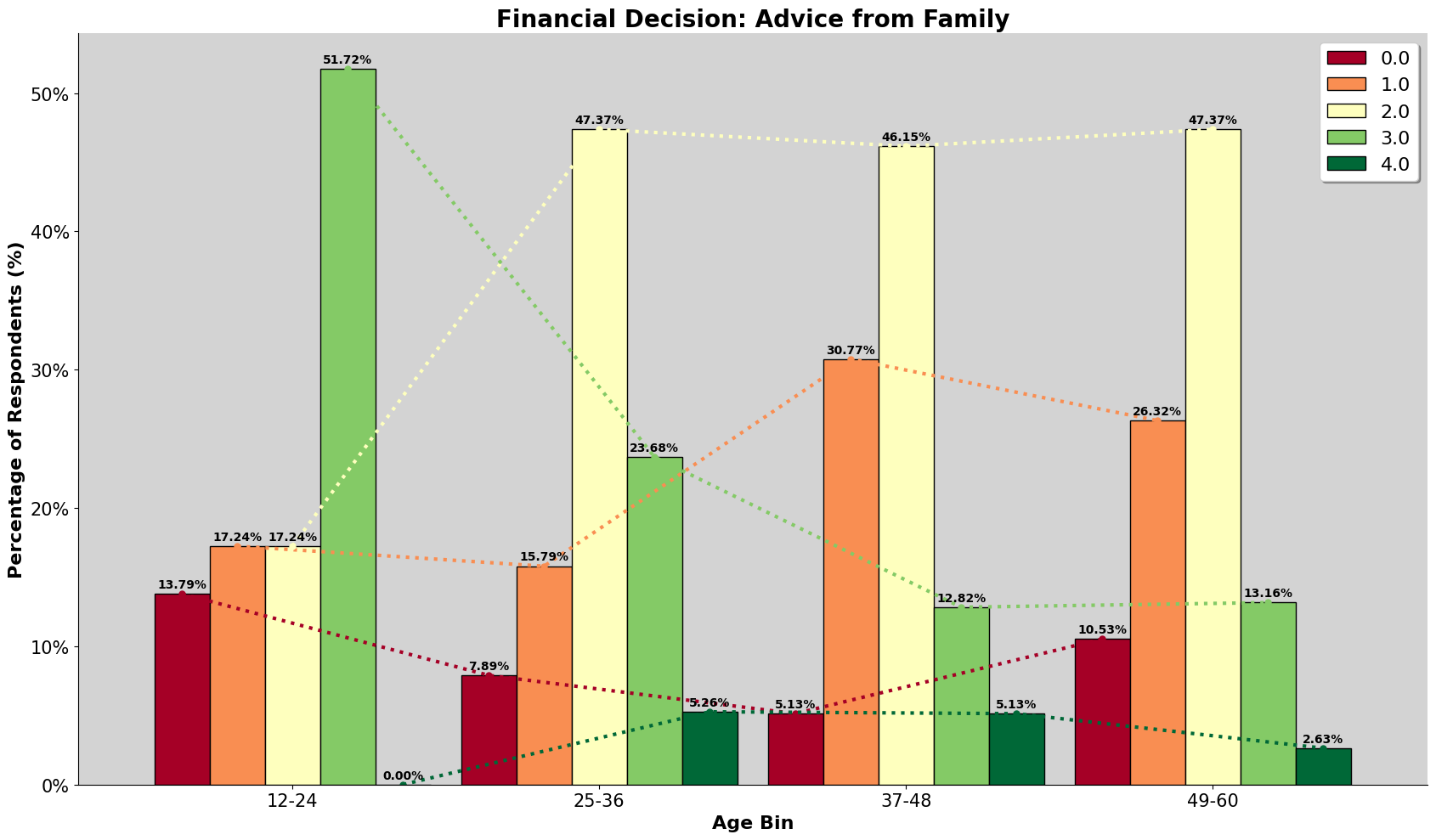
Based on the graph, we can see that there is an overwhelming half of the youngest age group rely on family for financial advice. The score of 3 then decreases as age group increases. The score of 2 remains about the same, and the score of 4 also decreases. However, we also see the score of 0 decreases but the score of 1 increases as age group increases. Overall, we can conclude that we rely on the advice of our family lesser as we grow older as we have learned and experienced more things on our own.
Financial Advisor across Age Groups - Who trusts the financial advisors more?
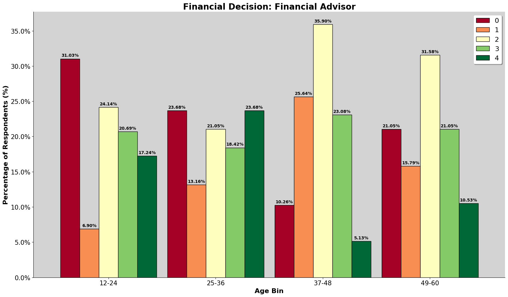
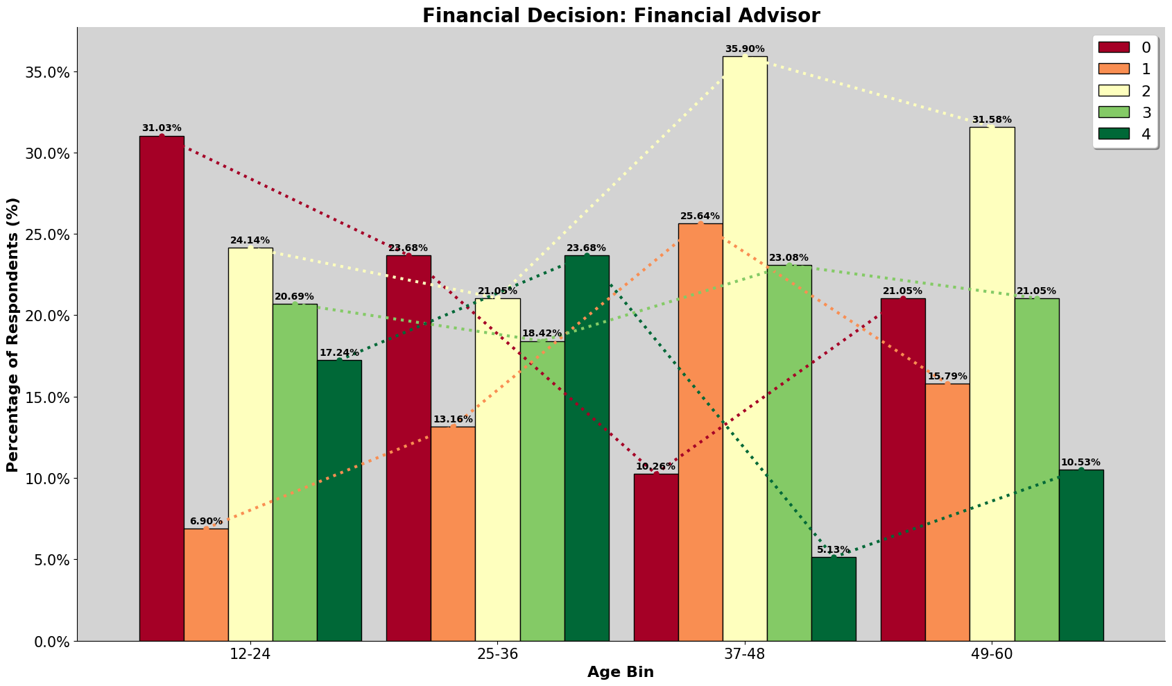
Based on the graph, there are no conclusive trend to be identified. Initially, we thought it is likelier for those who are middle-aged and older, who will hire financial advisors, as they can afford their services and have accumlated enough wealth for it to be manged optimally. It does seem to be the case at first, as we see a decrease in the score of 0 as age increases, but we also see this decrease in the score of 4.
Financial Advisor across Education Attainment - If you're already smart, do you still need an advisor?
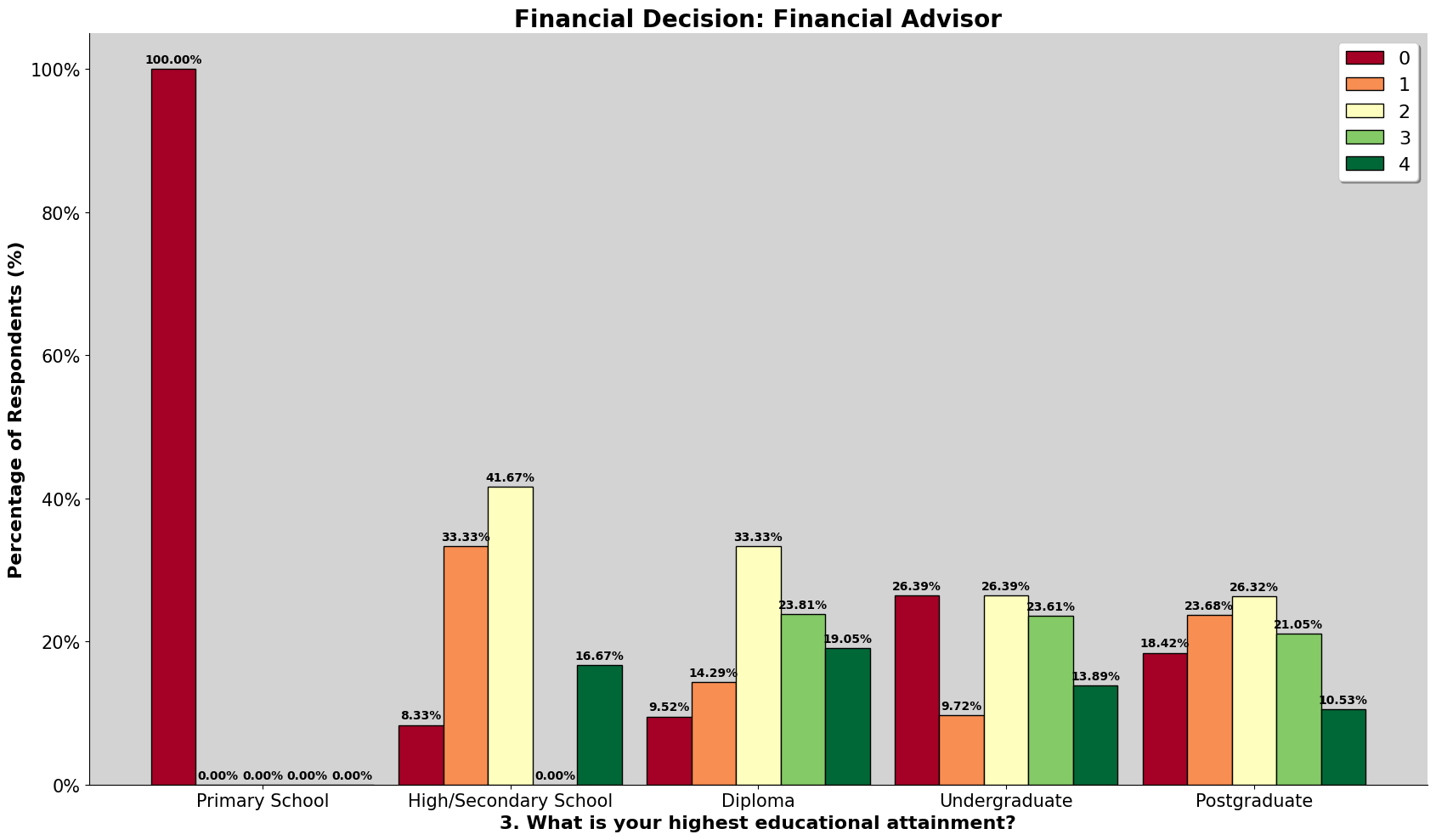
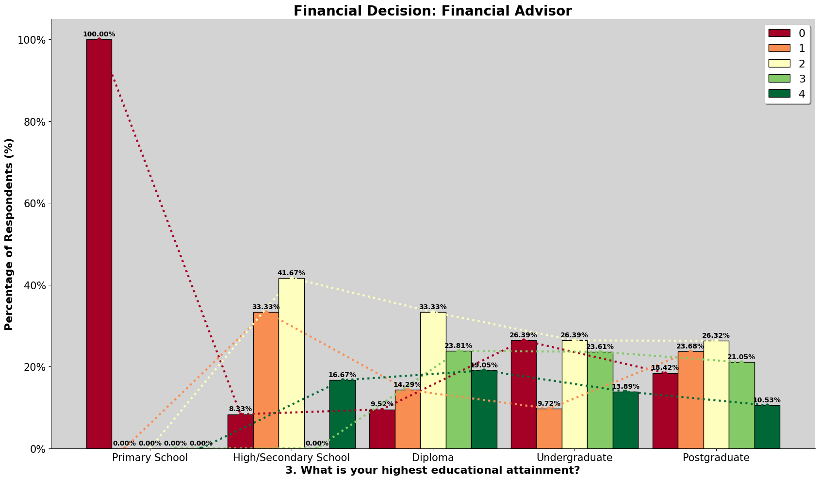
Based on the graph, we do observe a bit of a trend, where score of 0 and 1 increases as education attainment increases, and score of 2, 3 and 4 decreases. Therefore, ones' education attainment does reflect the trust in financial advisors.
We have also tried charting 'Financial Advisor' with 'Financial Literacy Score' and 'Income Range', thinking it might have some relationships such as having a higher financial literacy score will result in less likely of having a financial advisor, while if you had higher income, you would be able to hire one as you would have likely accumlated enough wealth that require optimal management. However, that was not the case and the graphs showed no visual identifiable pattern or relationship.
def create_financial_decision_graph(column_1, column_2, lineplot:bool=False):

    # Set Figure
    fig, ax = plt.subplots(figsize=(17,10))
    ax.set_facecolor('lightgrey')

    # Dataset
    df = our_dataset[[column_1, column_2]]\
        .groupby(column_1, observed=False).value_counts(normalize=True).sort_index()\
            .unstack()

    # Set width
    width=0.9

    # Set formatter
    formatter = mtick.PercentFormatter(xmax=1.0, decimals=None)

    # Plot bar
    df.plot(kind='bar', cmap='RdYlGn', rot=0, width=width, edgecolor='black', ax=ax)

    # Bar label
    for c in ax.containers:
        ax.bar_label(c, fmt='{:.2%}', fontsize=10, fontweight='bold', padding=3)

    # Plot lines
    if lineplot:
        n_groups = len(df)
        n_bars_per_group = len(df.columns)
        individual_bars_width = width / n_bars_per_group

        # Get the colormap to match line colors to bar colors
        color_set = [mpl.cm.RdYlGn(i / (n_bars_per_group - 1)) for i in range(n_bars_per_group)]

        for i, col_name in enumerate(df.columns):
            offset = (i - (n_bars_per_group - 1)/2) * individual_bars_width
            x_position = [p + offset for p in range(n_groups)]

            ax.plot(x_position, df[col_name], color=color_set[i],
                    marker='o', markersize=5, label='_nolegend_',
                    linestyle=':', linewidth=3)

    ax.set_title(column_2, fontsize=20, fontweight='bold')
    ax.set_xlabel(column_1, fontsize=16, fontweight='bold')
    ax.set_ylabel('Percentage of Respondents (%)', fontsize=16, fontweight='bold')
    ax.spines[['top', 'right']].set_visible(False)
    ax.legend(fontsize=16, shadow=True)
    ax.tick_params(axis='both', labelsize=15)
    ax.yaxis.set_major_formatter(formatter)

    plt.tight_layout()
    plt.show()

# Get column no
for col_no, col in enumerate(our_financial_decision_column_name):
    print(col_no, ' - ', col)

# Exploring Social Media

# - Age Bin
create_financial_decision_graph('Age Bin', our_financial_decision_column_name[3])
create_financial_decision_graph('Age Bin', our_financial_decision_column_name[3], True)

# - Education
create_financial_decision_graph(our_education_string, our_financial_decision_column_name[3])
create_financial_decision_graph(our_education_string, our_financial_decision_column_name[3], True)

# - Gender
create_financial_decision_graph(our_gender_string, our_financial_decision_column_name[3])

# Exploring Financial Advisor

# - Age Bin
create_financial_decision_graph('Age Bin', our_financial_decision_column_name[7])
create_financial_decision_graph('Age Bin', our_financial_decision_column_name[7], True)

# - Education
create_financial_decision_graph(our_education_string, our_financial_decision_column_name[7])
create_financial_decision_graph(our_education_string, our_financial_decision_column_name[7], True)

# Advice from friends

# - Age Bin
create_financial_decision_graph('Age Bin', our_financial_decision_column_name[4])
create_financial_decision_graph('Age Bin', our_financial_decision_column_name[4], True)
Correlations
Correlations for Romanian Dataset
Using the factors from the sections above, we will create a heatmap to explore the correlation of each of the factors against each other.
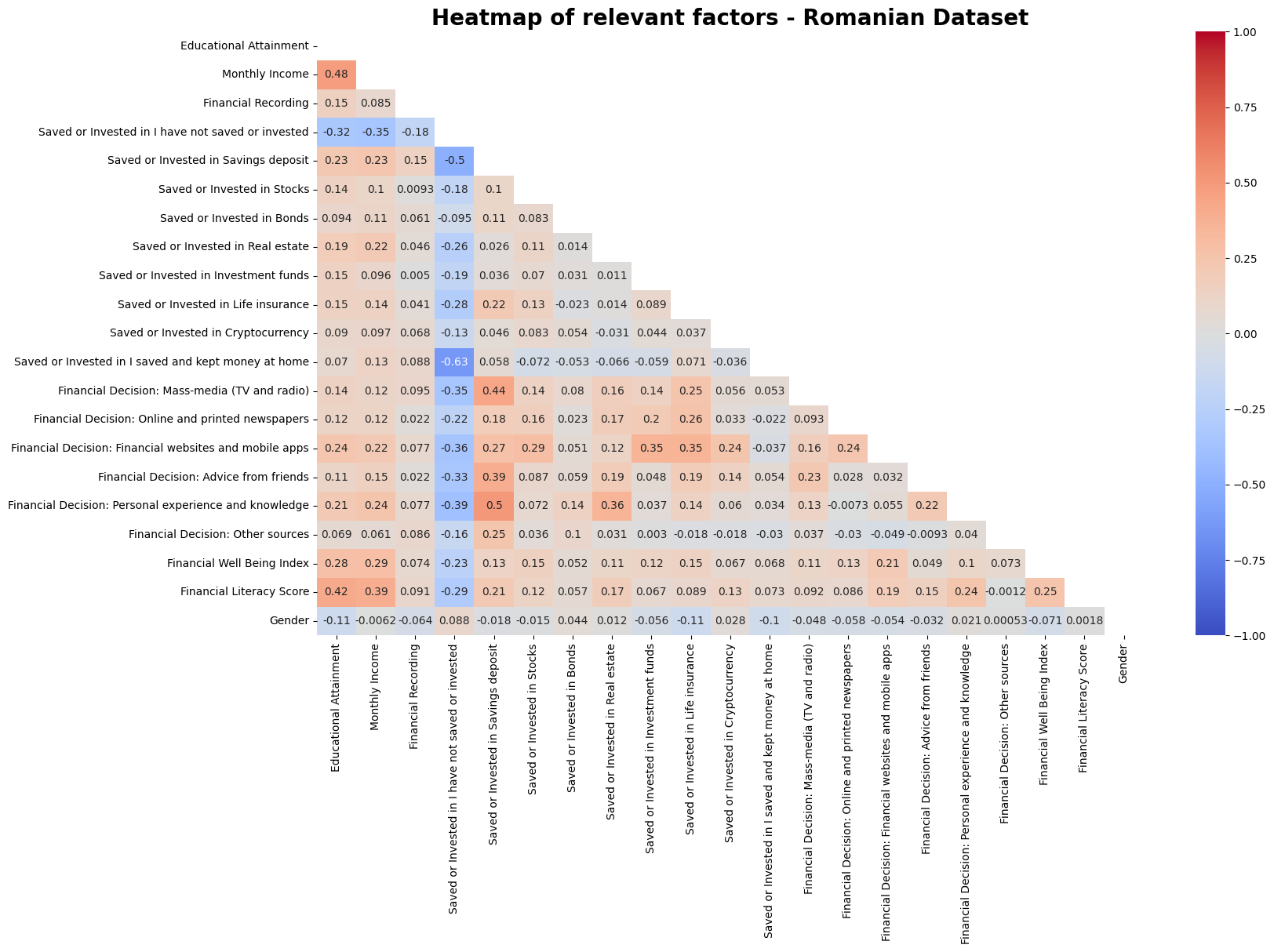
This heatmap is for the romanian dataset. Usually the heatmaps help us identify highly correlated pairs of factors by identifying those with deeper and more concentrated color. However, having quite a number of factors all on the graph can make it overwhelming to identify correlated pairs.
So the following is a list of the correlation in table form. The table below has been processed by turning the correlation into absolute values, as we would like find out the factor pairs that have higher affect on each other. Additionally, we have filter for those that have a correlation above 3. Else, the table would be too long.
| Correlation | |
|---|---|
| ('Saved or Invested in I saved and kept money at home', 'Saved or Invested in I have not saved or invested') | 0.634996 |
| ('Financial Decision: Personal experience and knowledge', 'Saved or Invested in Savings deposit') | 0.501465 |
| ('Saved or Invested in I have not saved or invested', 'Saved or Invested in Savings deposit') | 0.497124 |
| ('Educational Attainment', 'Monthly Income') | 0.479155 |
| ('Financial Decision: Mass-media (TV and radio)', 'Saved or Invested in Savings deposit') | 0.436049 |
| ('Financial Literacy Score', 'Educational Attainment') | 0.418181 |
| ('Financial Decision: Advice from friends', 'Saved or Invested in Savings deposit') | 0.394864 |
| ('Financial Literacy Score', 'Monthly Income') | 0.391294 |
| ('Saved or Invested in I have not saved or invested', 'Financial Decision: Personal experience and knowledge') | 0.390567 |
| ('Financial Decision: Personal experience and knowledge', 'Saved or Invested in Real estate') | 0.358448 |
| ('Financial Decision: Financial websites and mobile apps', 'Saved or Invested in I have not saved or invested') | 0.356151 |
| ('Financial Decision: Financial websites and mobile apps', 'Saved or Invested in Investment funds') | 0.35442 |
| ('Financial Decision: Financial websites and mobile apps', 'Saved or Invested in Life insurance') | 0.351923 |
| ('Financial Decision: Mass-media (TV and radio)', 'Saved or Invested in I have not saved or invested') | 0.349036 |
| ('Saved or Invested in I have not saved or invested', 'Monthly Income') | 0.348381 |
| ('Saved or Invested in I have not saved or invested', 'Financial Decision: Advice from friends') | 0.328616 |
| ('Saved or Invested in I have not saved or invested', 'Educational Attainment') | 0.323872 |
# Plot Figure
# ============
# Store the correlation matrix
romanian_dataset_subset_corr = romanian_dataset_subset.corr()

# Initialize the figure
figure, ax = plt.subplots(figsize=(17,10))

# Create a mask that covers the repeated portion of the matrix
mask = np.triu(np.ones_like(romanian_dataset_subset_corr, dtype=bool))

# Plot the heatmap
sns.heatmap(
    romanian_dataset_subset_corr,
    annot=True,
    cmap='coolwarm',
    vmin=-1,
    vmax=1,
    mask = mask,
    ax=ax)

# Title
plt.title("Heatmap of relevant factors - Romanian Dataset", size=20, weight='bold')

# Show the figure
plt.show()

# Table Form
# ==========
# Make values in the subset absolute, then sort it in descending order
temp_df = romanian_dataset_subset_corr.abs().unstack().sort_values(ascending=False)
temp_df = temp_df[temp_df<1] # Filter the those values that are 1
temp_df = temp_df.drop_duplicates() # Remove Duplicate values
temp_df = temp_df.to_frame('Correlation')
temp_df[temp_df['Correlation'] >= 0.3].to_markdown('romanian_correlation.md') # Export those that are above 3
Correlation for Our Dataset
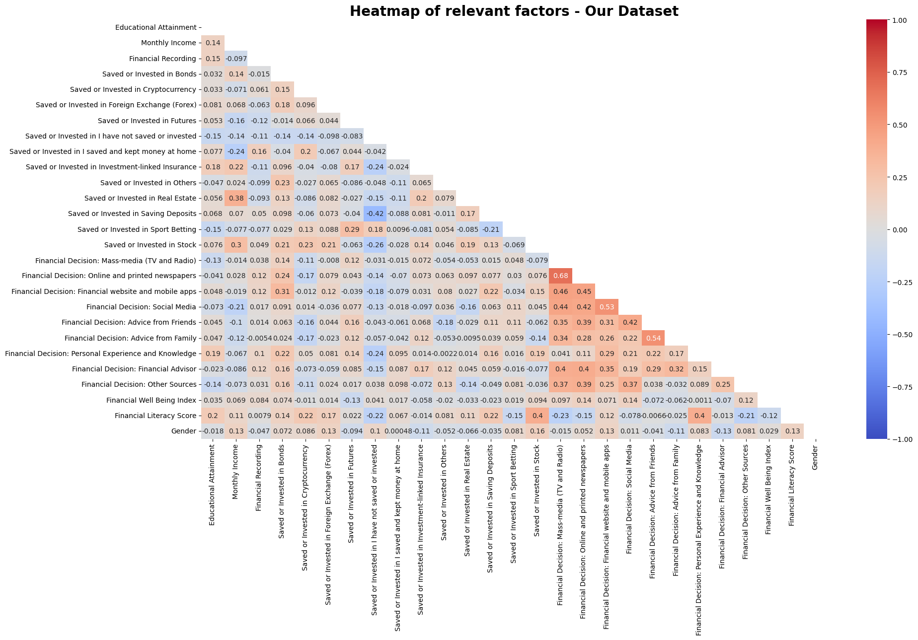
Similarly, the table form will be shown next with it being filtered for those that have absolute 0.3 and above.
| Correlation | |
|---|---|
| ('Financial Decision: Online and printed newspapers', 'Financial Decision: Mass-media (TV and Radio)') | 0.682066 |
| ('Financial Decision: Advice from Family', 'Financial Decision: Advice from Friends') | 0.544861 |
| ('Financial Decision: Social Media', 'Financial Decision: Financial website and mobile apps') | 0.532277 |
| ('Financial Decision: Mass-media (TV and Radio)', 'Financial Decision: Financial website and mobile apps') | 0.457382 |
| ('Financial Decision: Financial website and mobile apps', 'Financial Decision: Online and printed newspapers') | 0.447232 |
| ('Financial Decision: Social Media', 'Financial Decision: Mass-media (TV and Radio)') | 0.438903 |
| ('Financial Decision: Online and printed newspapers', 'Financial Decision: Social Media') | 0.424695 |
| ('Saved or Invested in Saving Deposits', 'Saved or Invested in I have not saved or invested') | 0.423262 |
| ('Financial Decision: Social Media', 'Financial Decision: Advice from Friends') | 0.415621 |
| ('Financial Decision: Financial Advisor', 'Financial Decision: Online and printed newspapers') | 0.400018 |
| ('Financial Literacy Score', 'Financial Decision: Personal Experience and Knowledge') | 0.398206 |
| ('Financial Decision: Mass-media (TV and Radio)', 'Financial Decision: Financial Advisor') | 0.39789 |
| ('Saved or Invested in Stock', 'Financial Literacy Score') | 0.395631 |
| ('Financial Decision: Advice from Friends', 'Financial Decision: Online and printed newspapers') | 0.391324 |
| ('Financial Decision: Other Sources', 'Financial Decision: Online and printed newspapers') | 0.386767 |
| ('Monthly Income', 'Saved or Invested in Real Estate') | 0.375496 |
| ('Financial Decision: Mass-media (TV and Radio)', 'Financial Decision: Other Sources') | 0.373191 |
| ('Financial Decision: Other Sources', 'Financial Decision: Social Media') | 0.368676 |
| ('Financial Decision: Advice from Friends', 'Financial Decision: Mass-media (TV and Radio)') | 0.351236 |
| ('Financial Decision: Financial Advisor', 'Financial Decision: Financial website and mobile apps') | 0.350085 |
| ('Financial Decision: Advice from Family', 'Financial Decision: Mass-media (TV and Radio)') | 0.336474 |
| ('Financial Decision: Advice from Family', 'Financial Decision: Financial Advisor') | 0.32061 |
| ('Saved or Invested in Bonds', 'Financial Decision: Financial website and mobile apps') | 0.314292 |
| ('Financial Decision: Financial website and mobile apps', 'Financial Decision: Advice from Friends') | 0.309425 |
The table for our dataset has more entries due to having more choices for participants to choose when it comes to the investing and financial decision influence. There are also more factors that have absolute correlation of more than 0.3.
# Plot Heatmap
# ==============
# Store the correlation matrix
our_dataset_subset_corr = our_dataset_subset.iloc[:,1:].corr()

# Initialize the figure
figure, ax = plt.subplots(figsize=(20,13))

# Create a mask that covers the repeated portion of the matrix
mask = np.triu(np.ones_like(our_dataset_subset_corr, dtype=bool))

# Plot the heatmap
sns.heatmap(
    our_dataset_subset_corr,
    annot=True,
    cmap='coolwarm',
    vmin=-1,
    vmax=1,
    mask = mask)

# Add title
plt.title("Heatmap of relevant factors - Our Dataset", size=20, weight='bold')

# Show the figure
plt.tight_layout()
plt.show()

# Table Form
# ===========
# Make values in the subset absolute, then sort it in descending order
temp_df = our_dataset_subset_corr.abs().unstack().sort_values(ascending=False)
temp_df = temp_df[temp_df<1] # Filter the those values that are 1
temp_df = temp_df.drop_duplicates() # Remove Duplicate values
temp_df = temp_df.to_frame('Correlation')
temp_df[temp_df['Correlation'] >= 0.3].to_markdown('our_correlation.md')
Correlation for Financial Well Being and Financial Literacy
The following are the correlation heatmap for only the financial well being and financial literacy score for the romanian dataset as well as the table form.
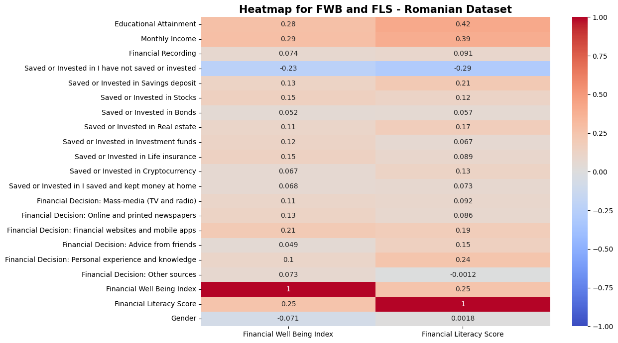
Financial Well Being Index Correlation for Romanian Dataset
| Correlation | |
|---|---|
| Financial Well Being Index | 1 |
| Monthly Income | 0.288022 |
| Educational Attainment | 0.275845 |
| Financial Literacy Score | 0.253676 |
| Saved or Invested in I have not saved or invested | 0.227974 |
| Financial Decision: Financial websites and mobile apps | 0.207159 |
| Saved or Invested in Stocks | 0.150847 |
| Saved or Invested in Life insurance | 0.145591 |
| Financial Decision: Online and printed newspapers | 0.128744 |
| Saved or Invested in Savings deposit | 0.126812 |
| Saved or Invested in Investment funds | 0.117687 |
| Saved or Invested in Real estate | 0.106827 |
| Financial Decision: Mass-media (TV and radio) | 0.10547 |
| Financial Decision: Personal experience and knowledge | 0.103033 |
| Financial Recording | 0.073752 |
| Financial Decision: Other sources | 0.0728505 |
| Gender | 0.0709994 |
| Saved or Invested in I saved and kept money at home | 0.068305 |
| Saved or Invested in Cryptocurrency | 0.0674963 |
| Saved or Invested in Bonds | 0.0523635 |
| Financial Decision: Advice from friends | 0.0487423 |
For financial well being for romanian dataset, the highest contributing factors would be Monthly Income, Education Attainment and Financial Literacy. Based on the section on Financial Well Being for the romanian dataset, we found that financial well being index were wide spread regardless of factors, and it can be seen here as well. While the top factors that could predict financial well being, only have correlation of below 0.3. Therefore, while it is highest among the factors listed, it is still not a strong correlation to financial well being.
Financial Literacy Correlation for Romanian Dataset
| Correlation | |
|---|---|
| Financial Literacy Score | 1 |
| Educational Attainment | 0.418181 |
| Monthly Income | 0.391294 |
| Saved or Invested in I have not saved or invested | 0.28929 |
| Financial Well Being Index | 0.253676 |
| Financial Decision: Personal experience and knowledge | 0.244754 |
| Saved or Invested in Savings deposit | 0.211959 |
| Financial Decision: Financial websites and mobile apps | 0.185982 |
| Saved or Invested in Real estate | 0.173152 |
| Financial Decision: Advice from friends | 0.150325 |
| Saved or Invested in Cryptocurrency | 0.125233 |
| Saved or Invested in Stocks | 0.118977 |
| Financial Decision: Mass-media (TV and radio) | 0.0923682 |
| Financial Recording | 0.0906506 |
| Saved or Invested in Life insurance | 0.0890882 |
| Financial Decision: Online and printed newspapers | 0.0857521 |
| Saved or Invested in I saved and kept money at home | 0.0729622 |
| Saved or Invested in Investment funds | 0.0669291 |
| Saved or Invested in Bonds | 0.0570054 |
| Gender | 0.00175718 |
| Financial Decision: Other sources | 0.00122341 |
As for the financial literacy for the romanian dataset, we can observe that Educaiton Attainment and Monthly Income have decent correlation to financial literacy, having 0.41 and 0.39 resepectively.
# Plot Heatmap
# =============
# Store the correlation matrix
romanian_dataset_subset_corr_fwbfl = romanian_dataset_subset_corr[romanian_dataset_subset.columns[18:20]]

# Initialize the figure
figure, ax = plt.subplots(figsize=(13,7))

# Plot the heatmap
sns.heatmap(
    romanian_dataset_subset_corr_fwbfl,
    annot=True,
    cmap='coolwarm',
    vmin=-1,
    vmax=1
    )

# Title
plt.title("Heatmap for FWB and FLS - Romanian Dataset", size=15, weight='bold')

# Show the figure
plt.tight_layout()
plt.show()

# Table Form
# ==========
# Get the absolute value, then sort the values in descending order
romanian_dataset_subset_corr_fwbfl_sorted = \
    romanian_dataset_subset_corr_fwbfl.abs().unstack()\
    .sort_values(ascending=False)

# Export the tables in markdown
romanian_dataset_subset_corr_fwbfl_sorted['Financial Literacy Score'].to_frame('Correlation').to_markdown('romanian_fls_cor.md')
romanian_dataset_subset_corr_fwbfl_sorted['Financial Well Being Index'].to_frame('Correlation').to_markdown('romanian_fwb_cor.md')
Now for our dataset.
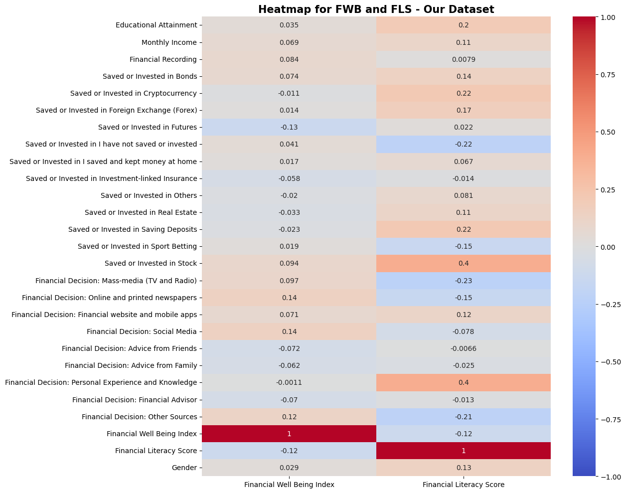
Financial Well Being Correlation for Our Dataset
| Correlation | |
|---|---|
| Financial Well Being Index | 1 |
| Financial Decision: Social Media | 0.144237 |
| Financial Decision: Online and printed newspapers | 0.141197 |
| Saved or Invested in Futures | 0.127223 |
| Financial Decision: Other Sources | 0.122909 |
| Financial Literacy Score | 0.11835 |
| Financial Decision: Mass-media (TV and Radio) | 0.0967151 |
| Saved or Invested in Stock | 0.0936123 |
| Financial Recording | 0.0837716 |
| Saved or Invested in Bonds | 0.0742211 |
| Financial Decision: Advice from Friends | 0.0722406 |
| Financial Decision: Financial website and mobile apps | 0.0713571 |
| Financial Decision: Financial Advisor | 0.0695535 |
| Monthly Income | 0.0689397 |
| Financial Decision: Advice from Family | 0.0620168 |
| Saved or Invested in Investment-linked Insurance | 0.0576237 |
| Saved or Invested in I have not saved or invested | 0.0405091 |
| Educational Attainment | 0.0353205 |
| Saved or Invested in Real Estate | 0.0327732 |
| Gender | 0.0294823 |
| Saved or Invested in Saving Deposits | 0.0232937 |
| Saved or Invested in Others | 0.0197731 |
| Saved or Invested in Sport Betting | 0.0190196 |
| Saved or Invested in I saved and kept money at home | 0.0169908 |
| Saved or Invested in Foreign Exchange (Forex) | 0.0143191 |
| Saved or Invested in Cryptocurrency | 0.0110185 |
| Financial Decision: Personal Experience and Knowledge | 0.0011145 |
Similarly to the romanian dataset, in the section on Financial Well Being, we also see that financial well being is widespread in terms of scoring regardless of any of the factors. The table above confirms it further, showing that all the factors only have a correlation of around 0.1. Ironically, it has a negative correlation with financial literacy score, though a weak one at -0.12. This shows that having a higher financial literacy, might cause financial well being to drop.
Financial Literacy Correlation for Our Dataset
| Correlation | |
|---|---|
| Financial Literacy Score | 1 |
| Financial Decision: Personal Experience and Knowledge | 0.398206 |
| Saved or Invested in Stock | 0.395631 |
| Financial Decision: Mass-media (TV and Radio) | 0.225691 |
| Saved or Invested in Cryptocurrency | 0.216893 |
| Saved or Invested in Saving Deposits | 0.21624 |
| Saved or Invested in I have not saved or invested | 0.215116 |
| Financial Decision: Other Sources | 0.212074 |
| Educational Attainment | 0.195647 |
| Saved or Invested in Foreign Exchange (Forex) | 0.168905 |
| Financial Decision: Online and printed newspapers | 0.153169 |
| Saved or Invested in Sport Betting | 0.148042 |
| Saved or Invested in Bonds | 0.139238 |
| Gender | 0.134631 |
| Financial Well Being Index | 0.11835 |
| Financial Decision: Financial website and mobile apps | 0.115469 |
| Saved or Invested in Real Estate | 0.113337 |
| Monthly Income | 0.106147 |
| Saved or Invested in Others | 0.0813299 |
| Financial Decision: Social Media | 0.077967 |
| Saved or Invested in I saved and kept money at home | 0.0674343 |
| Financial Decision: Advice from Family | 0.0245275 |
| Saved or Invested in Futures | 0.0217494 |
| Saved or Invested in Investment-linked Insurance | 0.0144798 |
| Financial Decision: Financial Advisor | 0.0127556 |
| Financial Recording | 0.00794666 |
| Financial Decision: Advice from Friends | 0.00658426 |
As for the financial literacy, we see that factors such as personal experience and knowledge, mass media as financial decision influence, and the act of investing in stocks, cryptocurrency, having saved in a saving deposit, have better correlation to financial literacy, than the factors we have explored. Hence, this shows the act of doing financial practices such as saving and investing, is a better predictor to financial literacy than education attainment, income and the other factors we have explored.
# Plot Heatmap
# =============
# Store the correlation matrix
our_dataset_subset_corr_fwbfl = our_dataset_subset_corr[our_dataset_subset.columns[25:27]]

# Initialize the figure
figure, ax = plt.subplots(figsize=(13,10))

# Plot the heatmap
sns.heatmap(
    our_dataset_subset_corr_fwbfl,
    annot=True,
    cmap='coolwarm',
    vmin=-1,
    vmax=1
    )

# Title
plt.title('Heatmap for FWB and FLS - Our Dataset', size=15, weight='bold')

# Show the figure
plt.tight_layout()
plt.show()

# Table Form
# ==========
# Get the absolute value, then sort the values in descending order
our_dataset_subset_corr_fwbfl_sorted = \
    our_dataset_subset_corr_fwbfl.abs().unstack()\
    .sort_values(ascending=False)

# Export as markdown
our_dataset_subset_corr_fwbfl_sorted['Financial Literacy Score'].to_frame('Correlation').to_markdown('our_fls_cor.md')
our_dataset_subset_corr_fwbfl_sorted['Financial Well Being Index'].to_frame('Correlation').to_markdown('our_fwb_cor.md')
Exploring those above the mean
We explore looking into factors, columns and characteristics for those that at least 1 standard deviation above the mean. We will do this by getting the mean for all columns and inspect the change to the mean.
The following function is to compare the mean of the general dataset and the filtered dataset. Then, the difference between the mean will be divided by the column's range (max value - min value), to get the true magnitude of the change in both dataset's mean. Why not use percentage? Because when we have used that method, and found that it is not indicative of the magnitude of the change. For example, there are columns of mean 2 decimal places. If they were to increase by the smallest amount, 0.005 to 0.01 is a 100% increase and it looks like a huge matter, but in actuality, 0.05 means almost no one is responding to a 1 to that question/feature/column. Hence, the change in mean is divided by the min and max value of the colum.
We will sort them based on change and note any observations
# Function used to generate table for mean comparison
# =====================================================
def list_changes_in_columns(new_dataset, dataset):

    # Set the column and DataFrame
    result_columns =  ['(+/-)', 'Change', 'Mean', 'New Mean', 'Column']
    result = pd.DataFrame(columns=result_columns)

    # Loop through the columns
    for col in new_dataset.columns:

        # Get the mean of the unfiltered dataset
        mean = round(dataset[col].mean(), 2)

        # Mean value of filtered dataset
        new_mean = round(new_dataset[col].mean(), 2)

        # Column min and max
        col_min = dataset[col].min()
        col_max = dataset[col].max()

        # True change value
        change = round(abs(new_mean - mean) / (col_max - col_min),2)

        # Store into a temp DataFrame
        temp = pd.DataFrame(
            {
                result_columns[0]:['+' if (new_mean > mean) else '-' ],
                result_columns[1]:[change],
                result_columns[2]:[mean],
                result_columns[3]:[new_mean],
                result_columns[4]:[col]
            }
        )

        # Combine the temp DataFrame with result
        result = pd.concat([result,temp],axis=0,ignore_index=True)

    return result

# Data Preparation
# =================
# Set the threshold based on the variable used above
romanian_financial_well_being_threshold = romanian_financial_well_being_mean + romanian_financial_well_being_std
our_financial_well_being_threshold = romanian_financial_well_being_mean + romanian_financial_well_being_std
romanian_financial_literacy_threshold = romanian_financial_literacy_mean + romanian_financial_literacy_std
our_financial_literacy_threshold = our_financial_literacy_mean + our_financial_literacy_std

# Set the conditions
romanian_financial_well_being_threshold_filter = \
    romanian_dataset_subset['Financial Well Being Index'] >= romanian_financial_well_being_threshold

our_financial_well_being_threshold_filter = \
    our_dataset_subset['Financial Well Being Index'] >= our_financial_well_being_threshold

romanian_financial_literacy_threshold_filter = \
    romanian_dataset_subset['Financial Literacy Score'] >= romanian_financial_literacy_threshold

our_financial_literacy_threshold_filter = \
    our_dataset_subset['Financial Literacy Score'] >= our_financial_literacy_threshold

romanian_financial_well_being_threshold_filter,our_financial_well_being_threshold_filter,romanian_financial_literacy_threshold_filter,our_financial_literacy_threshold_filter

# Financial Well Being - Romania
filter_by_financial_well_being_romanian = romanian_dataset_subset[romanian_financial_well_being_threshold_filter]
filter_by_financial_well_being_romanian_difference = list_changes_in_columns(filter_by_financial_well_being_romanian, romanian_dataset_subset)
filter_by_financial_well_being_romanian_difference.sort_values('Change', ascending=False).to_markdown('romanian_change_in_fwb.md')

# Financial Literacy - Romania
filter_by_financial_literacy_romania = romanian_dataset_subset[romanian_financial_literacy_threshold_filter]
filter_by_financial_literacy_romania_difference = list_changes_in_columns(filter_by_financial_literacy_romania, romanian_dataset_subset)
filter_by_financial_literacy_romania_difference.sort_values('Change', ascending=False).to_markdown('romanian_change_in_fls.md')

# Financial Well Being - Malaysia
filter_by_financial_well_being_our = our_dataset_subset[our_financial_well_being_threshold_filter].iloc[:,1:]
filter_by_financial_well_being_our_difference = list_changes_in_columns(filter_by_financial_well_being_our, our_dataset_subset)
filter_by_financial_well_being_our_difference.sort_values('Change',ascending=False).to_markdown('our_change_in_fwb.md')

# Financial Literacy - Malaysia
filter_by_financial_literacy_our = our_dataset_subset[our_financial_literacy_threshold_filter].iloc[:,1:]
filter_by_financial_literacy_our_difference = list_changes_in_columns(filter_by_financial_literacy_our, our_dataset_subset)
filter_by_financial_literacy_our_difference.sort_values('Change',ascending=False).to_markdown('our_change_in_fls.md')

# Combining the filters
combined_fl_fwb_filter_romanian = romanian_financial_well_being_threshold_filter & romanian_financial_literacy_threshold_filter
combined_fl_fwb_filter_our = our_financial_well_being_threshold_filter & our_financial_literacy_threshold_filter

# Both Filters Applied - Romania
print('Percentage of dataset when filtered by Financial Literacy: ',
      round(len(filter_by_financial_literacy_romania)/len(romanian_dataset)*100,2),'%')

print('Percentage of dataset when filtered by Financial Well Being: ',
      round(len(filter_by_financial_well_being_romanian)/len(romanian_dataset)*100, 2), '%')

print('Percentage of dataset when filtered by Both: ',
     round(len(romanian_dataset_subset[combined_fl_fwb_filter_romanian])/len(romanian_dataset)*100, 2), '%')

filter_by_fl_fwb_romanian = romanian_dataset_subset[combined_fl_fwb_filter_romanian]
filter_by_fl_fwb_romanian_difference = list_changes_in_columns(filter_by_fl_fwb_romanian,romanian_dataset_subset)
filter_by_fl_fwb_romanian_difference.sort_values('Change', ascending=False).to_markdown('romanian_change_in_fwbfls.md')

# Both Filters Applied - Malaysia
print('Percentage of dataset when filtered by Financial Literacy: ',
      round(len(filter_by_financial_literacy_our)/len(our_dataset)*100,2),'%')

print('Percentage of dataset when filtered by Financial Well Being: ',
      round(len(filter_by_financial_well_being_our)/len(our_dataset)*100, 2), '%')

print('Percentage of dataset when filtered by Both: ',
     round(len(our_dataset_subset[combined_fl_fwb_filter_our])/len(our_dataset)*100, 2), '%')
Change in Financial Well Being Mean - Romania Dataset
| (+/-) | Change | Mean | New Mean | Column | |
|---|---|---|---|---|---|
| 18 | + | 0.24 | 48.63 | 55.64 | Financial Well Being Index |
| 14 | + | 0.11 | 0.1 | 0.21 | Financial Decision: Financial websites and mobile apps |
| 3 | - | 0.08 | 0.53 | 0.45 | Saved or Invested in I have not saved or invested |
| 1 | + | 0.08 | 1.8 | 2.1 | Monthly Income |
| 9 | + | 0.07 | 0.06 | 0.13 | Saved or Invested in Life insurance |
| 0 | + | 0.05 | 2.35 | 2.54 | Educational Attainment |
| 19 | + | 0.05 | 2.74 | 3.14 | Financial Literacy Score |
| 12 | + | 0.05 | 0.1 | 0.15 | Financial Decision: Mass-media (TV and radio) |
| 20 | - | 0.05 | 0.48 | 0.43 | Gender |
| 5 | + | 0.05 | 0.03 | 0.08 | Saved or Invested in Stocks |
| 8 | + | 0.03 | 0.03 | 0.06 | Saved or Invested in Investment funds |
| 13 | + | 0.03 | 0.04 | 0.07 | Financial Decision: Online and printed newspapers |
| 4 | + | 0.03 | 0.18 | 0.21 | Saved or Invested in Savings deposit |
| 15 | - | 0.02 | 0.09 | 0.07 | Financial Decision: Advice from friends |
| 17 | + | 0.02 | 0.02 | 0.04 | Financial Decision: Other sources |
| 11 | - | 0.01 | 0.26 | 0.25 | Saved or Invested in I saved and kept money at home |
| 16 | + | 0.01 | 0.12 | 0.13 | Financial Decision: Personal experience and knowledge |
| 2 | + | 0.01 | 1.72 | 1.76 | Financial Recording |
| 10 | + | 0.01 | 0.02 | 0.03 | Saved or Invested in Cryptocurrency |
| 7 | - | 0 | 0.06 | 0.06 | Saved or Invested in Real estate |
| 6 | - | 0 | 0.01 | 0.01 | Saved or Invested in Bonds |
The table above shows the change in financial well being mean, when compared to those that are 1 standard deviation above the mean. The table is sorted based on the magnitude of the change in mean. We can see that those that have higher financial well being, tend to have an increase in having financial websites and mobiles apps be their financial decision influence. We also see that there is an increase in monthly income, education, financial literacy score, and mass media as financial decision.
Change in Financial Literacy - Romanian Dataset
| (+/-) | Change | Mean | New Mean | Column | |
|---|---|---|---|---|---|
| 19 | + | 0.33 | 2.74 | 5.38 | Financial Literacy Score |
| 3 | - | 0.18 | 0.53 | 0.35 | Saved or Invested in I have not saved or invested |
| 1 | + | 0.13 | 1.8 | 2.34 | Monthly Income |
| 0 | + | 0.12 | 2.35 | 2.82 | Educational Attainment |
| 4 | + | 0.11 | 0.18 | 0.29 | Saved or Invested in Savings deposit |
| 16 | + | 0.11 | 0.12 | 0.23 | Financial Decision: Personal experience and knowledge |
| 14 | + | 0.08 | 0.1 | 0.18 | Financial Decision: Financial websites and mobile apps |
| 7 | + | 0.07 | 0.06 | 0.13 | Saved or Invested in Real estate |
| 15 | + | 0.06 | 0.09 | 0.15 | Financial Decision: Advice from friends |
| 20 | + | 0.06 | 0.48 | 0.54 | Gender |
| 18 | + | 0.04 | 48.63 | 49.82 | Financial Well Being Index |
| 2 | + | 0.04 | 1.72 | 1.83 | Financial Recording |
| 12 | + | 0.03 | 0.1 | 0.13 | Financial Decision: Mass-media (TV and radio) |
| 5 | + | 0.03 | 0.03 | 0.06 | Saved or Invested in Stocks |
| 9 | + | 0.02 | 0.06 | 0.08 | Saved or Invested in Life insurance |
| 11 | - | 0.02 | 0.26 | 0.24 | Saved or Invested in I saved and kept money at home |
| 10 | + | 0.02 | 0.02 | 0.04 | Saved or Invested in Cryptocurrency |
| 8 | + | 0.01 | 0.03 | 0.04 | Saved or Invested in Investment funds |
| 6 | + | 0.01 | 0.01 | 0.02 | Saved or Invested in Bonds |
| 17 | + | 0.01 | 0.02 | 0.03 | Financial Decision: Other sources |
| 13 | - | 0 | 0.04 | 0.04 | Financial Decision: Online and printed newspapers |
Similarly, we see that those that have at least 1 standard deviation above the financial literacy mean, there is an increase in monthly income, edcation attainment, savings in deposit, relying personal experience for financial decision, relying on financial websites and mobile apps for financial decisions and having saved/invested in real estate.
Change in Financial Well Being Mean - Our Dataset
| (+/-) | Change | Mean | New Mean | Column | |
|---|---|---|---|---|---|
| 24 | + | 0.32 | 48.64 | 54.81 | Financial Well Being Index |
| 22 | - | 0.16 | 1.91 | 1.25 | Financial Decision: Financial Advisor |
| 7 | + | 0.15 | 0.1 | 0.25 | Saved or Invested in I have not saved or invested |
| 23 | + | 0.13 | 0.55 | 1.06 | Financial Decision: Other Sources |
| 8 | + | 0.13 | 0.18 | 0.31 | Saved or Invested in I saved and kept money at home |
| 25 | - | 0.12 | 4.59 | 3.75 | Financial Literacy Score |
| 18 | + | 0.12 | 1.51 | 2 | Financial Decision: Social Media |
| 10 | - | 0.11 | 0.11 | 0 | Saved or Invested in Others |
| 11 | - | 0.11 | 0.17 | 0.06 | Saved or Invested in Real Estate |
| 9 | - | 0.1 | 0.41 | 0.31 | Saved or Invested in Investment-linked Insurance |
| 26 | + | 0.09 | 0.58 | 0.75 | Gender |
| 3 | - | 0.09 | 0.15 | 0.06 | Saved or Invested in Bonds |
| 4 | - | 0.09 | 0.15 | 0.06 | Saved or Invested in Cryptocurrency |
| 12 | - | 0.08 | 0.7 | 0.62 | Saved or Invested in Saving Deposits |
| 14 | - | 0.07 | 0.38 | 0.31 | Saved or Invested in Stock |
| 16 | + | 0.06 | 1.43 | 1.69 | Financial Decision: Online and printed newspapers |
| 0 | + | 0.05 | 2.93 | 3.12 | Educational Attainment |
| 15 | + | 0.05 | 1.31 | 1.5 | Financial Decision: Mass-media (TV and Radio) |
| 1 | - | 0.04 | 2.94 | 2.75 | Monthly Income |
| 13 | + | 0.03 | 0.03 | 0.06 | Saved or Invested in Sport Betting |
| 17 | - | 0.02 | 1.81 | 1.75 | Financial Decision: Financial website and mobile apps |
| 19 | + | 0.02 | 1.85 | 1.94 | Financial Decision: Advice from Friends |
| 21 | - | 0.02 | 2.51 | 2.44 | Financial Decision: Personal Experience and Knowledge |
| 5 | - | 0.02 | 0.08 | 0.06 | Saved or Invested in Foreign Exchange (Forex) |
| 2 | + | 0.02 | 1.56 | 1.62 | Financial Recording |
| 20 | + | 0.01 | 1.9 | 1.94 | Financial Decision: Advice from Family |
| 6 | - | 0 | 0.06 | 0.06 | Saved or Invested in Futures |
As for our dataset, for those that have at least 1 standard deviation above the financial well being mean, ironically, there is actually a decrease in having financial advisor for financial decision advise, decrease in financial literacy, decrease in investment in real estate. Additionally, there is also an increase for those that do not save or invest. We also see a decrese in investing in Bonds, Cryptocurrency, and in stocks. This is a baffling finding as it goes against the notion that we need to optimize our excess cash in investements and other means in order to further generate wealth for our financial well being.
We also noted earlier in the financial well being across gender section, we intially observed that there are no differences between male or female when it comes to financial well being. However, based on our table result, we see that there is an increase in the gender (from 0.58 to 0.75, 0 indicating female and 1 indicating male), which indicates that on average there are financial well being that are at least 1 standard deviation above the mean has more males.
Change in Financial Literacy - Our Dataset
| (+/-) | Change | Mean | New Mean | Column | |
|---|---|---|---|---|---|
| 25 | + | 0.34 | 4.59 | 7 | Financial Literacy Score |
| 14 | + | 0.29 | 0.38 | 0.67 | Saved or Invested in Stock |
| 21 | + | 0.26 | 2.51 | 3.56 | Financial Decision: Personal Experience and Knowledge |
| 4 | + | 0.24 | 0.15 | 0.39 | Saved or Invested in Cryptocurrency |
| 12 | + | 0.19 | 0.7 | 0.89 | Saved or Invested in Saving Deposits |
| 3 | + | 0.18 | 0.15 | 0.33 | Saved or Invested in Bonds |
| 2 | - | 0.11 | 1.56 | 1.22 | Financial Recording |
| 17 | + | 0.1 | 1.81 | 2.22 | Financial Decision: Financial website and mobile apps |
| 5 | + | 0.09 | 0.08 | 0.17 | Saved or Invested in Foreign Exchange (Forex) |
| 15 | - | 0.08 | 1.31 | 1 | Financial Decision: Mass-media (TV and Radio) |
| 26 | + | 0.05 | 0.58 | 0.67 | Gender |
| 19 | + | 0.05 | 1.85 | 2.06 | Financial Decision: Advice from Friends |
| 7 | - | 0.04 | 0.1 | 0.06 | Saved or Invested in I have not saved or invested |
| 20 | - | 0.04 | 1.9 | 1.72 | Financial Decision: Advice from Family |
| 23 | - | 0.03 | 0.55 | 0.44 | Financial Decision: Other Sources |
| 0 | + | 0.03 | 2.93 | 3.06 | Educational Attainment |
| 13 | + | 0.03 | 0.03 | 0.06 | Saved or Invested in Sport Betting |
| 1 | - | 0.02 | 2.94 | 2.83 | Monthly Income |
| 18 | - | 0.02 | 1.51 | 1.44 | Financial Decision: Social Media |
| 9 | - | 0.02 | 0.41 | 0.39 | Saved or Invested in Investment-linked Insurance |
| 16 | - | 0.01 | 1.43 | 1.39 | Financial Decision: Online and printed newspapers |
| 22 | + | 0.01 | 1.91 | 1.94 | Financial Decision: Financial Advisor |
| 8 | - | 0.01 | 0.18 | 0.17 | Saved or Invested in I saved and kept money at home |
| 24 | + | 0.01 | 48.64 | 48.83 | Financial Well Being Index |
| 11 | - | 0 | 0.17 | 0.17 | Saved or Invested in Real Estate |
| 10 | - | 0 | 0.11 | 0.11 | Saved or Invested in Others |
| 6 | - | 0 | 0.06 | 0.06 | Saved or Invested in Futures |
As for financial literacy, we see similar results to the romanian dataset, where having invested in financial instruments like bonds, stocks, cryptocurreny, saving deposits or forex and relying on personal experience and knowledge for financial decisions is a better indicator if some one has high financial literacy. As if one does, they would likely be participating and understand the complexity of investment and financial management. However, paradoxically, we see a decrease in financial recording behaviour.
As for financial well being, we can see that having at least 1 standard deviation above the mean financial literacy, does increase financial well being, but only a little.
Combining filters - those that have above Financial Literacy and Financial Well Being
We now filter for those that are at least 1 standard deviation above the mean for financial literacy and financial well being. When filtering only for one condition in the romanian dataset, there are about 16.46% and 13.08% of the dataset left, for financial literacy and financial well being respectively. When we filtered for both, only 3.09% of the dataset remanins.
| (+/-) | Change | Mean | New Mean | Column | |
|---|---|---|---|---|---|
| 19 | + | 0.32 | 2.74 | 5.33 | Financial Literacy Score |
| 3 | - | 0.27 | 0.53 | 0.26 | Saved or Invested in I have not saved or invested |
| 18 | + | 0.25 | 48.63 | 55.77 | Financial Well Being Index |
| 1 | + | 0.21 | 1.8 | 2.63 | Monthly Income |
| 14 | + | 0.2 | 0.1 | 0.3 | Financial Decision: Financial websites and mobile apps |
| 16 | + | 0.14 | 0.12 | 0.26 | Financial Decision: Personal experience and knowledge |
| 0 | + | 0.13 | 2.35 | 2.86 | Educational Attainment |
| 5 | + | 0.11 | 0.03 | 0.14 | Saved or Invested in Stocks |
| 4 | + | 0.1 | 0.18 | 0.28 | Saved or Invested in Savings deposit |
| 9 | + | 0.1 | 0.06 | 0.16 | Saved or Invested in Life insurance |
| 2 | + | 0.09 | 1.72 | 2 | Financial Recording |
| 7 | + | 0.06 | 0.06 | 0.12 | Saved or Invested in Real estate |
| 17 | + | 0.05 | 0.02 | 0.07 | Financial Decision: Other sources |
| 20 | + | 0.05 | 0.48 | 0.53 | Gender |
| 13 | + | 0.03 | 0.04 | 0.07 | Financial Decision: Online and printed newspapers |
| 15 | + | 0.03 | 0.09 | 0.12 | Financial Decision: Advice from friends |
| 11 | - | 0.03 | 0.26 | 0.23 | Saved or Invested in I saved and kept money at home |
| 10 | + | 0.03 | 0.02 | 0.05 | Saved or Invested in Cryptocurrency |
| 8 | + | 0.02 | 0.03 | 0.05 | Saved or Invested in Investment funds |
| 12 | - | 0.01 | 0.1 | 0.09 | Financial Decision: Mass-media (TV and radio) |
| 6 | + | 0.01 | 0.01 | 0.02 | Saved or Invested in Bonds |
So the above table is the filtered for both financial well being and financial literacy. Ironically, we see a decrease for those that saves. We also see a decrease in those that kept money at home, and relying mass media for their financial decision. Everything else such as factors like monthly income, education, financial recording behaviour, investing in stocks, and savings deposits, seem to increase with having increased financial literacy and financial well being.
For our dataset, when we filtered for those that are at least 1 standard deviation above the mean for financial literacy and financial well being, there were 12.5% and 11.11%, respectively. But when we filtered for both, there were only 0.69% left. That is basically 1 person.
Does possessing financial literacy lead to financial well being?
Based on the above analysis, when we filtered those that have financial literacy of 1 standard deviation above the mean for the romanian dataset, we observed that the financial well being increase, as indicated by the increase in the mean value of the subset dataset from the main dataset. When we filter for those that have 1 standard deviation above the mean for financial well being, we also noted that financial literacy also increased. Therefore, financial literacy does positively affect financial well being. We will use the paired t test to see if it is statiscally significant.
stats, p_value = ttest_ind(
    romanian_dataset_subset['Financial Well Being Index'],
    romanian_dataset_subset['Financial Literacy Score']
)

if p_value < 0.05:
    print('The two columns are statistically significant')
else:
    print('The two columns are not statistically significant')
The two columns are statistically significantFor our dataset on the other hand, when we have filtered with for those having financial literacy of 1 standard deviation above mean, we can observe that financial well being increased barely. The mean value went from 48.64 to 48.83. Additionally, when we filtered for those with higher financial well being, we can see that the mean value of financial literacy actually dropped from 4.59 to 3.75. Therefore, based on our dataset and these analysis, we cannot say that having financial literacy will lead to financial well being.
We will test for the if they are statistically significant, to further substantiate our point.
stats, p_value = ttest_ind(
    our_dataset_subset['Financial Well Being Index'],
    our_dataset_subset['Financial Literacy Score']
)

if p_value < 0.05:
    print('The two columns are statistically significant')
else:
    print('The two columns are not statistically significant')
The two columns are statistically significantTherefore, for the romanian dataset, it is clear that financial literacy does indeed contribute to having better financial well being, but for our dataset, it is the contrary. While it is statistically significant, it financial literacy does not neccessarily bring financial well being.
Conclusions
We have used an external dataset along with our own dataset. We have made comparison throughout the project and was managed to cover all the research objectives and questions. We understood that even though the general education attainment level of Romania is at high school while Malaysia have commonly have undergraduate, there were instances of financial literacy in Romania scored higher than participants in Malaysia, while Malaysia still had the higher mean financial literacy. Similarly, even though it seems that the Malaysian dataset had percentage of individuals who make higher end of monthly income, but financial well being were still lower as compared to the Romania dataset. We also compared some sociodemographic attributes along with other such as monthly income and the habit of financial recording arranged in the age group and noted some trends. We also found out that Romania consists slightly more than half of the dataset, do not save nor invest, while about 70% of Malaysian dataset at least save in a saving deposit. Some comparison such as the financial decision influence, due to change in survey question and structure, it has made the comparison not accurate.
Financial well being and financial literacy were computed using several columns. With this, we compared both dataset and noted that Malaysia seem to have lower well being and literacy scores. But this could also be due to the insufficient samples for this survey to be effective. We then explore most of the columns and its affect with financial literacy and financial well being. We noted that for the romanian dataset, the main sociodemographic features that likely increase financial well being and financial literacy are education attaiment, monthly income, age and whether they save / invest or not, while for the Malaysia dataset, had contradictory findings. We done this comparison by changes in mean value with the general dataset and the filter dataset for those with higher financial well being or financial literacy. We also used correlation to find the relationship between features.
We also explore if financial well being and financial literacy affect each other for Romanian dataset, while the Malaysian dataset, had contradictory results once again. Those with higher Financial Literacy, tend to have lower Financial Well Being. We also found that financial literacy increase the percevied risk of the HRFV in part 2. But, the same group of individuals, also participated anyways, especially Cryptocurrency, where financial literacy have a big effect for it. Therefore, financial literacy can encourage an individual to get into it. Rather than avoiding it.
Note that we were supposed to explore our survey with the Ghanaian Study but it now feels like it is out of scope as well as the time constraint. Some justifications for adopting the study for this survey are written in the appendix.
Requirements
# List of Imports
from matplotlib import pyplot as plt
import matplotlib as mpl
import numpy as np
import pandas as pd
import seaborn as sns
from textwrap import wrap
from scipy.stats import ttest_ind
from matplotlib.gridspec import GridSpec
import matplotlib.ticker as ticker
import matplotlib.ticker as mtick
References
Akhter, A., Sangmi, M.-D., 2016. Relationship between financial literacy and personal financial wellbeing - an empirical study. Abhigyan 34, 37–46.
Ali, A., Rahman, M.S.A., Bakar, A., 2015. Financial Satisfaction and the Influence of Financial Literacy in Malaysia. Soc Indic Res 120, 137–156. https://doi.org/10.1007/s11205-014-0583-0
Goyal, K., Kumar, S., 2021. Financial literacy: A systematic review and bibliometric analysis. Int J Consum Stud. https://doi.org/10.1111/ijcs.12605
Hii, I.S.H., Ho, P.L., Yap, C.S., Philip, A.P., 2022. Financial Literacy, Financial Advice, and Stock Market Participation: Evidence From Malaysia. Journal of Financial Counseling and Planning 33, 243–254. https://doi.org/10.1891/JFCP-2021-0011
Kah, Y., Chung, C., Fenn, J., Abdulraqeb, A., Al-Khaled, S., 2021. The Relationship between Socio-Demographics and Financial Literacy with Financial Planning Among Young Adults in Klang Valley, Malaysia (Hubungan Antara Sosio-Demografi dan Literasi Kewangan dengan Perancangan Kewangan dalam Kalangan Belia di Klang Valley, Malaysia). Jurnal Pengurusan 63. https://doi.org/10.17576/pengurusan-2021-63-02
Lusardi, A., Mitchell, O.S., 2009. NBER WORKING PAPER SERIES HOW ORDINARY CONSUMERS MAKE COMPLEX ECONOMIC DECISIONS: FINANCIAL LITERACY AND RETIREMENT READINESS.
McGee, D., 2020. On the normalisation of online sports gambling among young adult men in the UK: a public health perspective. Public Health 184, 89–94. https://doi.org/10.1016/j.puhe.2020.04.018
Nițoi, M., Clichici, D., Zeldea, C., Pochea, M., Ciocîrlan, C., 2022. Financial well-being and financial literacy in Romania: A survey dataset. Data Brief 43. https://doi.org/10.1016/j.dib.2022.108413
Nyemcsok, C., Pitt, H., Kremer, P., Thomas, S.L., 2022. Young men’s perceptions about the risks associated with sports betting: a critical qualitative inquiry. BMC Public Health 22. https://doi.org/10.1186/s12889-022-13164-2
Ofosu, A., Kotey, R.A., 2019. Does Sports Betting Affect Investment Behaviour? Evidence from Ghanaian Sports Betting Participants.
Rahman, M., Isa, C.R., Masud, M.M., Sarker, M., Chowdhury, N.T., 2021. The role of financial behaviour, financial literacy, and financial stress in explaining the financial well-being of B40 group in Malaysia. Future Business Journal 7. https://doi.org/10.1186/s43093-021-00099-0
Statista (2023), Total Employment in Malaysia from 2012 to 2021. Available at: https://www.statista.com/statistics/621259/employment-in-malaysia/#:~:text=In 2021%2C approximately 15 million,country was around 68.6 percent. (Accessed: 30 May 2023)
Statista (2023), Number of students enrolled in public higher education institutions in Malaysia from 2012 to 2020, by gender. Available at: https://www.statista.com/statistics/794845/students-in-public-higher-education-institutions-by-gender-malaysia/#:~:text=In 2020%2C around 234.08 thousand,than male students in 2019. (Accessed: 30 May 2023)
World Bank (2023), Available at: https://data.worldbank.org/country/malaysia?view=chart (Accessed: 30 May 2023)
World Bank (2023), Available at: https://data.worldbank.org/indicator/NY.GDP.MKTP.CD?locations=GH (Accessed: 30 May 2023)
Yang, M., Al Mamun, A., Mohiuddin, M., Ali Al-Shami, S.S., Zainol, N.R., 2021. Predicting stock market investment intention and behavior among malaysian working adults using partial least squares structural equation modeling. Mathematics 9. https://doi.org/10.3390/math9080873
Zhang, Y., Chatterjee, S., 2023. Financial Well-Being in the United States: The Roles of Financial Literacy and Financial Stress. Sustainability 2023, Vol. 15, Page 4505 15, 4505. https://doi.org/10.3390/SU15054505
Zhao, H., Zhang, L., 2021. Financial literacy or investment experience: which is more influential in cryptocurrency investment? International Journal of Bank Marketing 39, 1208–1226. https://doi.org/10.1108/IJBM-11-2020-0552
Zulfiqar, M., Bilal, M., 2016. Financial Wellbeing is the Goal of Financial Literacy, Research Journal of Finance and Accounting www.iiste.org ISSN. Online.
Appendix
Differences / Changes made to the Questions (Change Log)
The following are the questions that we have used in the survey mapped to the questions used in the other studies. This will be useful when referring to the columns from both survey. Justification for the changes that have been made to the survey and answers are stated in the section below for the Romanian Study and for the Ghanaian study.
List of Questions - Part I - Sociodemographic Variables
| No. | Questions | Romanian Study Questions | Romanian Study No. |
|---|---|---|---|
| - | - | Please indicate your residential status | SD1 |
| 1 | What is your gender? | Please indicate the gender of the respondent | SD2 |
| 2 | What is your age? | What is your age (completed years)? | SD3 |
| 3 | What is your highest educational attainment? | What is your highest educational attainment? | SD4 |
| 4 | What is your current employment status? | What is your current employment status? | SD5 |
| 5 | How many people, including yourself, live permanently in your household? | How many persons, including yourself, live permanently in your household? | SD6 |
| 6 | What is your monthly income after tax? | What is your monthly income after taxes? | SD7 |
| 7 | What is your marital status | Please indicate your marital status? | SD8 |
| 8 | Do you have a current bank account? | Do you have a current bank account? | SD9 |
List of Questions - Part II - Financial Behaviour and Attitudes
| No. | Question | Romanian Study Questions | Romanian Study No. |
|---|---|---|---|
| 9 | Do you or other person in your household keep a record of income and expenses on a monthly basis? | Do you or other person in your household keep a record of income and expenses on a monthly basis? | I1 |
| 10 | In the past three years, have you saved or invested money in any of the following instruments? Select those that applies. | In the past three years, have you saved or invested money in any of the following instruments? | I2 |
| 10.a | If Which of the following represents a barrier in saving or investing? | Which of the following represents a barrier in saving or investing money? | I4 |
| 10.a.1 | Lack of Money | Lack of Money | I4_1 |
| 10.a.2 | Lack of Time | Lack of Time | I4_2 |
| 10.a.3 | Lack of Financial Knowledge | Lack of Financial | I4_3 |
| - | - | Access to Financial Education Programs | I4_4 |
| 11 | Which of the following sources do you use to influence your financial decisions? Not only in investing | Which of the following sources do you use to support your financial decisions? | I3 |
| 11.1 | Mass-Media (TV and Radio) | Mass-media (TV and Radio) | I3_1 |
| 11.2 | Online and printed newspaper | Online and printed newspaper | I3_2 |
| 11.3 | Financial websites and mobile apps | Financial websites and mobile apps | I3_3 |
| 11.4 | Social Media | - | - |
| 11.5 | Advice from friends | Advice from friends | I3_4 |
| 11.6 | Advice from family | - | - |
| 11.7 | Personal experience and knowledge | Personal experience and knowledge | I3_5 |
| 11.8 | Finance Advisor | - | - |
| 11.9 | Other sources | Other sources | I3_6 |
| - | - | Which of the following phrases apply to you | I5 |
| 12 | Which of the following organizations do you see the most suitable to deliver financial education programs in your country? | Which of the following organizations do you see the most suitable to deliver financial education programs in Romania? | I6 |
| 12 | Commercial banks, insurance companies, pension funds, investment funds | Commercial banks, insurance companies, pension funds, investment funds | I6_1 |
| 12 | Non-government organizations | Non-government organizations | I6_2 |
| 12 | Regulators and Government | National Bank of Romania, Financial Supervisory Authority, National Authority for Consumer Protection | I6_3 |
| 12 | Higher education institutions | Higher education institutions | I6_4 |
| 12 | Mass Media | Mass Media | I6_5 |
| 12 | Other | Other | I6_6 |
| 12 | None of the above | None of the above | I6_7 |
| 12 | Don't know | Don't know | I6_8 |
| 13 | What financial concepts you wish were taught in high school or university as a compulsory subject? | What financial concepts would you be interested in receiving information free of charge? | I7 |
| 13 | Interest rates on loans and deposit | Interest rates on loans and deposit | I7_1 |
| 13 | Stocks, bonds, and investment funds | Stocks, bonds, and investment funds | I7_2 |
| 13 | Real Estate | Real Estate | I7_3 |
| 13 | Cryptocurrency | Cryptocurrency | I7_4 |
| 13 | Macroeconomic indicators (inflation rate, nominal interest rate, real interest rate, GDP) | Macroeconomic indicators (inflation rate, nominal interest rate, real interest rate, GDP) | I7_5 |
| 13 | Changes in the level of minimum wage, public pensions, social benefits, taxes | Changes in the level of minimum wage, public pensions, social benefits, taxes | I7_6 |
| 13 | I am not interested | I am not interested | I7_0 |
| 13 | Other | - | - |
List of Questions - Part III - Financial Well-Being
| No. | Question | Romanian Study Question | Romanian Study No. |
|---|---|---|---|
| 14 | How well does this statement describe you or your situation | How well does this statement describe you or your situation? | A |
| 14.1 | I could handle a major unexpected expense | I could handle a major unexpected expense | A1_1 |
| 14.2 | I am securing my financial secure | I am securing my financial future. | A1_2 |
| 14.3 | Because of my money situation, I feel like i will never have the things I want in life | Because of my money situation, I feel like I will never have the things I want in life. | A1_3 |
| 14.4 | I can enjoy life because of the way I am managing my money | I can enjoy life because of the way I’m managing my money | A1_4 |
| 14.5 | I am just getting by financially | I am just getting by financially | A1_5 |
| 14.6 | I am concerned that the money I have or will save will not last. | I am concerned that the money I have or will save won’t last | A1_6 |
| 15 | How often does this statement apply to you? | How often does this statement apply to you? | B |
| 15.1 | Giving a gift for a wedding, birthday or other occasion would put a strain on my finances for the month | Giving a gift for a wedding, birthday or other occasion would put a strain on my finances for the month | B1_1 |
| 15.2 | I have money left over at the end of the month | I have money left over at the end of the month | B1_2 |
| 15.3 | I am behind with my finances | I am behind with my finances | B1_3 |
| 15.4 | My finances control my life | My finances control my life. | B1_4 |
List of Questions - Part IV - Financial Literacy
| No. | Question | Romanian Study Question | Romanian Study No |
|---|---|---|---|
| 16 | Which of the following represents the highest probability | Which of the following represents the highest probability of something happening? | C1 |
| 17 | Suppose you had $100 in a savings account and the interest rate was 10 percent per year. After 5 years, how much do you think you would have in the account if you left the money to grow | Suppose you had LEI 100 in a savings account and the interest rate was 10 percent per year. After 5 years, how much do you think you would have in the account if you left the money to grow? | C2 |
| 18 | True or false: A 15-year mortgage typically requires higher monthly payments than a 30-year mortgage but the total interest over the life of the loan will be less | True or false: A 15-year mortgage typically requires higher monthly payments than a 30-year mortgage but the total interest over the life of the loan will be less. | C3 |
| 19 | Assume a friend inherits $50,000 now, and his sibling inherits $50,000, 3 years from now. Who is richer because of the inheritance? | Assume a friend inherits LEI 50,000 and his sibling inherits LEI 50,000 3 years from now. Who is richer because of the inheritance? | C4 |
| 20 | Suppose over the next 10 years the prices of things you buy double. If your income also doubles, will you be able to buy less than you can buy today, the same as you can buy today, or more than you can buy today? | Suppose over the next 10 years the prices of things you buy double. If your income also doubles, will you be able to buy less than you can buy today, the same as you can buy today, or more than you can buy today? | C5 |
| 21 | Suppose you have some money. It is safer to put your money into one business or investment, or to put your money into multiple businesses or investments? | Suppose you have some money. It is safer to put your money into one business or investment, or to put your money into multiple businesses or investments? | C6 |
| 22 | Considering a long time period (for example, 10 or 20 years), which asset normally gives the highest return? | Considering a long time period (for example, 10 or 20 years), which asset normally gives the highest return? | C7 |
| 23 | Normally, which asset displays the highest fluctuations over time? | Normally, which asset displays the highest fluctuations over time? | C8 |
Changes from the Romanian Study
This change log consists of the rationale for the changes made from the original questionnaire performed in the reference studies. The changes listed below, will need to be addressed when preparing and pre-processing the data. Therefore, it also serves as a checklist on what areas need to be matched before using the analyzing the data together.
The two reference studies that are mentioned here are
Note: This part of the content is best used alongside with the list of questions for the survey. It would also be complementary to have the reference study’s list.
Part I: Sociodemographic Variables
-
The first question was removed because the population of survey is highly likely to be in an urban are with over 100,000 people. The survey will be performed on the population in Kuala Lumpur. Instead, it will be asking the survey participants if that are from Malaysia.
-
The distinction between “primary school (4 grades)”, “middle school (8 grades)” and “high school (12 grades)” in the reference study were clearer and was split into 3 choices. This was changed into choices of “primary school” and “high/secondary school” in this project, because the structure of education here in the target countries. There are major exams at 12 years old (equivalent to a grade 6), and 16/17 years old (equivalent to a grade 12). The choice of “diploma” into the choice as it is also one popular option for both Malaysians and Singaporeans to pursue after their high school education.
-
Rewording changes. From the “Not working” to “Unemployed”. It is also rearranged. The “Not working” position swapped with the “Retired”.
-
Rather than using a fixed set of ranges like the one in the reference study, we want would like to have the participant state the amount. This would give us the freedom to analyze and explore the different possible ranges.
After sending out the survey for some people to do, their feedback was that having specific income typed out, is too invasive and felt too private to share, so having it in a range should help better. -
Consensual union has been removed as it is not a popular practice and there are no laws or regulations in Malaysia and Singapore that specifically recognize or provide legal status for consensual unions.
Part II: Financial Behaviour and Attitudes
-
In the reference study, they have allowed survey participants to choose only up to 3 choices. For our study, we have allowed survey participants to choose any of those that are relevant, whichever applies to them. This will give us even more insight into the importance of the what is saved and invested. Furthermore, not only have we rearranged the choices but added additional choices for survey participants to choose. The following are the addition choices that have been added: Foreign Exchange (Forex), Futures, Options, Sports Betting and Others. This was added to expand the selection and increase specificity. There is also rewording from “Life insurance” to “Investment-linked Insurance”, because life insurance alone does not seem like a viable way to act as an investment vehicle. The increase of choices was also done because the target audience that we wanted to survey are highly likely to have invested and might even have more 1 outlet of saving and investing.
-
In the reference study, they have allowed survey participants to choose only up to 2 of the answers. For our study, we have made participants to rank the choices based on the likert scale. Similar to above, this will give us more insight and increase specificity in what can be observed. Additional option of “Social Media” and “Advice from Family has also been added because the two added option are viable options that are not in the selection list.
-
In the reference study, there are 4 options as to what represents the barrier or difficulty in saving or investing money. For our study, we have removed the fourth option of “Access to Financial Education programs” because this options and the third option of “Lack of Financial Knowledge” seem to be same. It is because there is lack of reliable access to financial education program or sources in which will cause lack of financial knowledge. Furthermore, this is a question that only appears for those that have selected the choice of “I saved and kept money at home” and “I have not saved or invested” in question 2 of this section. But it will be rearranged below the intended question, rather than like the one in the reference study, where it will only appear after question 3 when this is supposed to be related to question 2. The question only appears for those who do not invest and do not save, when they pick the option of “I have not saved or invested” or “I saved and kept money at home”.
-
In the reference study, it seems that have a tendency to have educational program as an option and it feels out of place. Furthermore, we believe that the distinction and intention of each statement are not obvious enough. For example, the options:
a. I prefer to invest in activities that I can directly control.
b. I prefer to invest in other types of activities, e.g., educational programs.
c. I consider that investing in stocks is risky.
d. I consider that savings deposit is the safest investment
The option a. and b. are similar, so as c. and d. A person who prefers to invests in activities that they can control can be activities such as investing into education program and self-improvement. Even though, investing in activities that I can directly control can be other activities and not only in educational programs. As for c. and d., both statements are too similar. Even though there are still options such as government bonds and index funds, which are in between the risk of savings deposit and stocks, but if you share the sentiment that stock is too risky, it is highly likely that you would share the sentiment that saving in a deposit account is the safest option.
Therefore, we have removed this question for the questionnaire.
-
In the reference study, there is an option where they have listed the Romanian regulators and government body, “National Bank of Romania, Financial Supervisory Authority, National Authority for Consumer Protection”. For our study, we have simplified the to “Regulators and Government”, as our intention of sending the survey for Malaysians and Singaporeans, listing down all the relevant parties would just create unnecessary lengths in the answer.
-
For our study, we have rephrased the question from “What financial concepts would you be interested in receiving information free of charge?” to “What financial concepts you wish were taught in high school or university as a compulsory subject?”. This is because if a person is motivated to learn regarding these topics, they would and will be able to use the internet as a tool for learning the subject matter. But if we place emphasis on being a compulsory subject in school, then it is not only free content, but it becomes something that everyone must learn and will have some exposure to such knowledge. We wanted to add additional options of all the higher risk financial vehicles, but chose not to because it would be an overwhelming constantly having many choices from one question to another.
Part III: Financial Well-Being
No changes were made to this part of the questionnaire.
Part IV: Financial Literacy
Changed the currency from LEI to a dollar sign, $. That way, it is generic and understandable by any participants for all the questions being asked in this part of the questionnaire.
Part V: Views on High-Risk Financial Vehicles
This part of the questionnaire is referenced and based of another paper.
-
Because the study is only focused on sport-betting, it only questions on whether sport betting is risky or not. But for our study, we are looking into understanding their views for not only sport betting, but the other financial instruments as well.
-
Similarly, the answer to the question has been customized to be more general to higher risk investments rather than sport betting. Even though, sport betting is also part of it. The reference study also had 5 options with 1 being “No response”. As for our study, it is in our view that the intention of the question was to understand what the participant would do with the money. But the presented options in the reference study are as follows. Investing anything else, spending all the money, betting all the money, bet half the money and save half the money. It can be observed that the choices are extreme where their participants can either spend all money, or invest all money, or put all into sport betting, with one answer being half into sport-betting and half to save. For our study, we will give participant the choice of lower risk investments such as fixed deposits, government bills or bonds, and higher risk investments such as Cryptocurrency, Options, Forex, Futures, Sport-betting. The choices will then be, all in either choices, half in both choices or more than half in either choice. We also included the choice of “I would most likely spend it all” and also “Not sure what to do with it”.
-
Because sport-betting is not the only choice among the high-risk financial vehicle. This question does not feel as relevant. Giving a hypothetical amount to stop the action might not be applicable to other of the higher-risk financial vehicle.
-
Before asking participants, the upcoming questions based on the reference study, we thought to include to ask if they have personally experience or use any of the high-risk financial vehicle. It will only be more accurate if they have experience in being exposed to it.
Changes with the Ghanaian Study
As shown above, the changes that were made to accommodate the topic of choice for this project. We used this as reference study because of the topic and that the question structure seem fitting for the scope of the project.
The questions that were asked in Ghanaian study are listed below:
-
Do you see sports betting as very risky or not?
- Yes, it is very risk
- No, it is not
- No response
-
If you had GHC 10,000, what would you do with it?
- I would invest it in treasury bills or other investments
- I would most likely spend it
- I will bet it on sports so I would triple the money
- I would save half and bet the rest on sports
-
If you are asked to stop sports betting and receive GHC 10,000, would you do it?/
- Yes, I would
- No, I would not
- No response
-
How do you feel when participating in sports betting?
- I feel great
- I feel anxious
- I feel confident
- I feel very scared
- No response
-
Do you have any investments elsewhere?
- No, sports is my only investments
- Yes, I have investments elsewhere and I use the profits to bet on sports
- Yes, I have other investments because I do not need one
- No response
-
Which of the following are you able to do more because of betting?
- I am able to save more from my betting gains
- I spend more of my money on betting, one day I will win big
- I am able to have a more fulfilling and happier even though I do not win all my bets
- No response.
The changes that we have made are listed below.
-
We have applied this question to all the HRFV, but it only appears if participants were to have select that they have invest or save with the instrument before. We also implemented a likert scale rather than binary choice, just in case if it can support certain findings and the freedom of having more values to be process or formed later on.
-
Changed the currency and the amount to adapt to current audience. Rearranged the choices to have an arbitrary scale. Started with spending it all. Then, 'I would invest all into higher risk investments' is adapted from 'I would bet it on sports so I would triple the money'. We have removed the reason at the back, 'so i could tripple the money', because that could make the answer a little too outstanding and make participant unconsciously pick it. Then added the option of half invest into lower risk investment, as to have some from of gradient, or a spectrum to the finding.
-
Skipped as the question felt pointless after asking something similar already.
-
This is implemented similar to 1., where only if participants answer that they have invested with the particular instrument, then the question will pop up.
-
Included another choice to make the answer transition better from one choice to the next better.
List of Questions - Higher Risk Financial Vehicle and Ghana Sport Betting Study
| No. | Questions | Ghanaian Study Questions |
|---|---|---|
| 24 | What are your views on risk involved in the following financial instruments? | Do you see sport betting as very risk or not? |
| 25 | If you had $100,000 as a gift, what would you do with it given the following options? Lower risk investments: Fixed deposits, Government bills or Bonds. Higher risk investments: Cryptocurrency, Options, Forex, Futures, Sport-betting | If you had GHC 10,000, what would you do with it? |
| 26 | Have you invested or used any of the higher-risk financial vehicle? Select those that you have been exposed to before. | - |
| 26.a | How do you feel when participating <HRFV chosen by participant> | How do you feel when participating in sports betting? |
| 26.f | Which of the following says more about you? | Which of the following are you able to do more because of betting? |
| 26.g | Do you have any other investments elsewhere, other than the listed higher risk financial vehicle? | Do you have any investment elsewhere? |
| 26.h | Do you have investments elsewhere, that are not the list of higher risk financial vehicle listed in the survey? | - |
Financial Well Being Score Table
Scoring a total response value will given a final score of the column in the right. Therefore, scoring 27 on the questionnaire, will result of having a final score of 59.
| Total Response Value | Questionnaire Self - Administered |
|---|---|
| 0 | 14 |
| 1 | 19 |
| 2 | 22 |
| 3 | 25 |
| 4 | 27 |
| 5 | 29 |
| 6 | 31 |
| 7 | 32 |
| 8 | 34 |
| 9 | 35 |
| 10 | 37 |
| 11 | 38 |
| 12 | 40 |
| 13 | 41 |
| 14 | 42 |
| 15 | 44 |
| 16 | 45 |
| 17 | 46 |
| 18 | 47 |
| 19 | 49 |
| 20 | 50 |
| 21 | 51 |
| 22 | 52 |
| 23 | 54 |
| 24 | 55 |
| 25 | 56 |
| 26 | 58 |
| 27 | 59 |
| 28 | 60 |
| 29 | 62 |
| 30 | 63 |
| 31 | 65 |
| 32 | 66 |
| 33 | 68 |
| 34 | 69 |
| 35 | 71 |
| 36 | 73 |
| 37 | 75 |
| 38 | 78 |
| 39 | 81 |
| 40 | 86 |
Financial Well Being Questionnaire Value Representation
A, How well does this statement describe you or your situation?
A1_1 I could handle a major unexpected expense
| Completely | 4 |
| Very well | 3 |
| Somewhat | 2 |
| Very little | 1 |
| Not at all | 0 |
A1_ 2. I am securing my financial future.
| Completely | 4 |
| Very well | 3 |
| Somewhat | 2 |
| Very little | 1 |
| Not at all | 0 |
A1_3. Because of my money situation, I feel like I will never have the things I want in life.
| Completely | 0 |
| Very well | 1 |
| Somewhat | 2 |
| Very little | 3 |
| Not at all | 4 |
A1_4. I can enjoy life because of the way I’m managing my money.
| Completely | 4 |
| Very well | 3 |
| Somewhat | 2 |
| Very little | 1 |
| Not at all | 0 |
A1_5. I am just getting by financially.
| Completely | 0 |
| Very well | 1 |
| Somewhat | 2 |
| Very little | 3 |
| Not at all | 4 |
A1_6. I am concerned that the money I have or will save won’t last.
| Completely | 0 |
| Very well | 1 |
| Somewhat | 2 |
| Very little | 3 |
| Not at all | 4 |
B. How often does this statement apply to you?
B1_1. Giving a gift for a wedding, birthday or other occasion would put a strain on my finances for the month.
| Always | 0 |
| Often | 1 |
| Sometimes | 2 |
| Rarely | 3 |
| Never | 4 |
B1_2. I have money left over at the end of the month.
| Always | 4 |
| Often | 3 |
| Sometimes | 2 |
| Rarely | 1 |
| Never | 0 |
B1_3. I am behind with my finances.
| Always | 0 |
| Often | 1 |
| Sometimes | 2 |
| Rarely | 3 |
| Never | 4 |
B1_10. My finances control my life.
| Always | 0 |
| Often | 1 |
| Sometimes | 2 |
| Rarely | 3 |
| Never | 4 |
We will need to convert the values accordingly.