Abstract
In this project, we were able to explore the two most common investment strategy, 'Buy and Hold' and 'Dollar Cost Averaging' and our simple proposed models. The result is that if an investor is willing to take some risk and explore options outside of index funds, 'Dollar Cost Averaging' could be beneficial, especially if the stock is very volatile. Our proposed methods while there were instances where they managed outperformed both these strategies, it might not be worth the risk and effort required.
We have also looked into ways how we could prepare the data in various configurations for different uses such as having it used for data analysis or future studies where we would like to explore machine learning solutions for pattern recognition.
Note that all the values might change as they use the values of the last 730 days of data.
Libraries Required
The following are the required libraries. It is highly likely that required to download and install the 'yfinance' library.
Installing yfinance
%pip install yfinanceRequirement already satisfied: yfinance in ...
...
Note: you may need to restart the kernel to use updated packages.Importing Libraries
import numpy as np
from matplotlib import pyplot as plt
import pandas as pd
import yfinance as yf
Aims and Objective
Aim
The aim of the project is to explore if investing strategies supported with the use of machine learning techniques, can outperform the simple investing strategies, such as 'buy and hold', 'cost dollar averaging' and 'index fund investing', and simple trading strategies derived form data analysis.
Objectives
The objective of the project is to:
- To create simple investment strategies using traditional methods of data analysis
- To create investment strategies supported by machine learning techniques
- To compare the all the different proposed strategies to see which can perform best
- To explore which investment strategy can outperform the simple baseline strategies
- Explore if combining these strategies would make a better investing strategy, like an ensemble of decision makers.
The aim and objectives set at the start were definitely ambitious. Machine learning supported strategies were not explored in this coursework.
Investment Strategies
Firstly, we will need to understand some context to the strategies that are being used as the base comparisons. The following are brief description of what each strategies do. These strategies acts as a baseline that our proposed strategies will need to beat to be a successful strategy. We will then proceed to demonstrate and calculate the performance of these strategies.
Buy and Hold
The easiest strategy that everyone can do without any experience or expertise, is to "buy and hold". This means that the investors or market participants, purchase a financial instrument, for the case of our project, it would be stock, and not sell it. Selling it after the price has appreciated or increased, will result in a profit while selling it if the price is lower than it is initially bought, would result in a loss.
Dollar Cost Averaging
This strategy is very similar to "buy and hold", but rather than immediately purchasing the stock from day 1, dollar cost averaging employs an interval based purchase over a period of time. This is a popular strategy because most people do not have the time and proper strategy in place to take advantage of the daily price movement of the market. Hence, by buying stock at a set interval, for example, every week. This will allow the investor to potentially buy into the market, at a better time. The downside of it is that, investor might also be buying a stock at a bad time.
Index Fund Investing
This is a strategy that is endorsed and supported by the famous investor, Warren Buffet. This strategy involves buying the most diversified stock, the index fund. Index funds are a financial instrument that functions a lot like stock, but rather than only exposing to a single company or business, investors will be expose to the average of many businesses. There are many types of index funds and they are usually country specific. The S&P500, which allows investors to get exposure of the top 500 companies in the US, is one the most well known index fund. This index fund is also widely used as a benchmark in gauging investment performance. The 'Buy and Hold' and 'Dollar Cost Average' strategy will also be applied.
Investment Strategies Baseline Performance and Illustrations
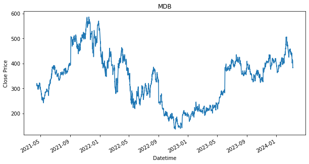
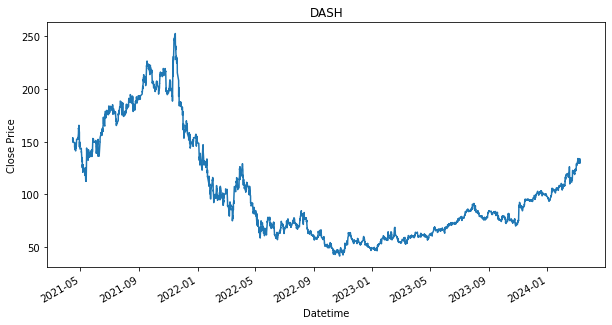
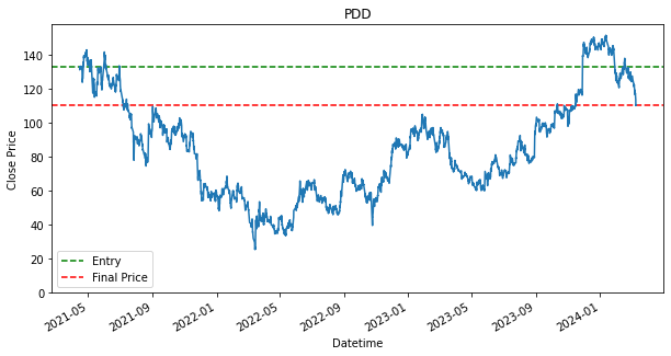
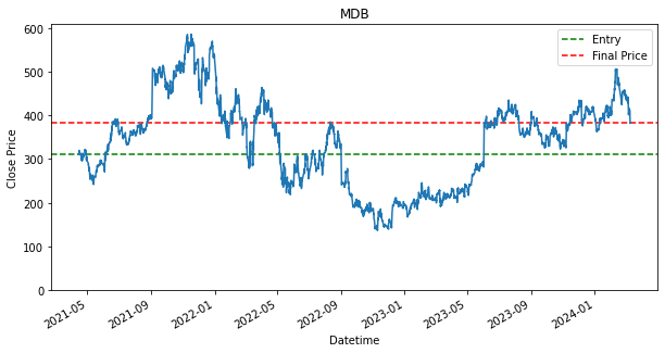
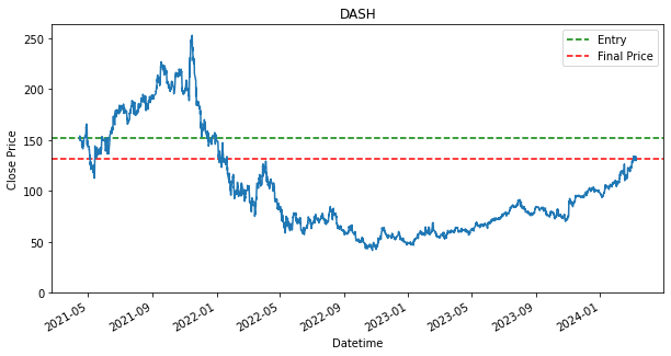
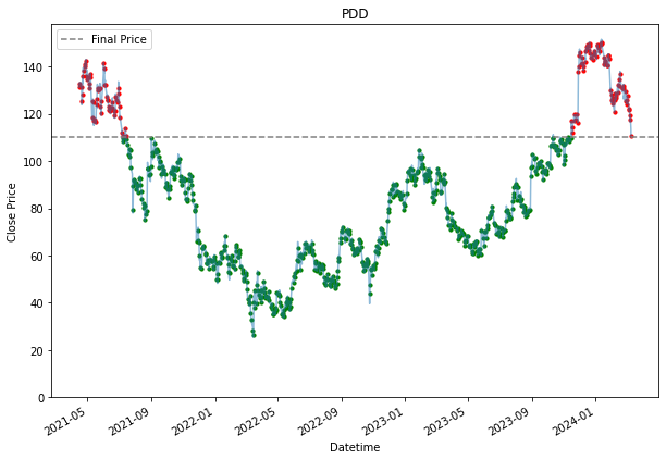
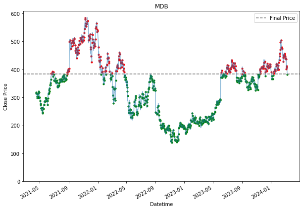
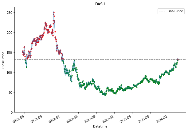
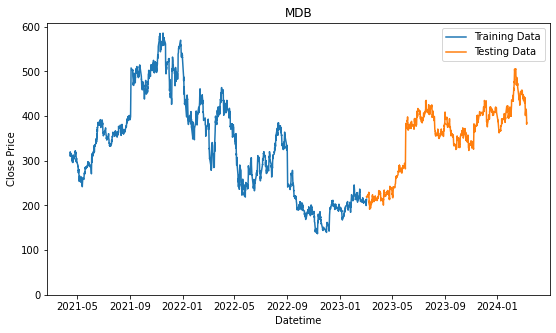
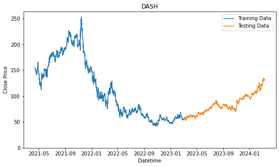
Now, we will look into all of the performances based on the strategies above. We will be using data that was mentioned in the previous coursework, when we have selected the top 3 highest price moving company, among the Nasdaq100 in the technology sector using evaluation criteria that was also presented in the previous coursework. The companies were Pinduoduo Inc (PDD), Mongodb Inc (MDB), and DoorDash Inc (DASH). The bracketed values are their stock ticker, which is a short formed text used to identify the stock on various of platforms.
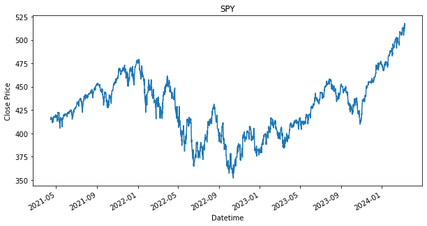
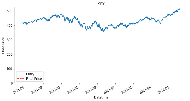
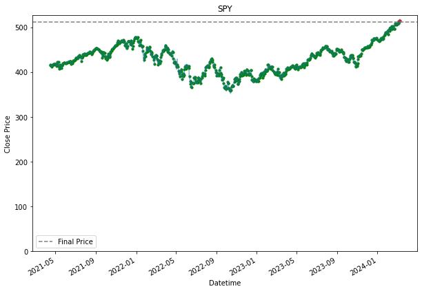
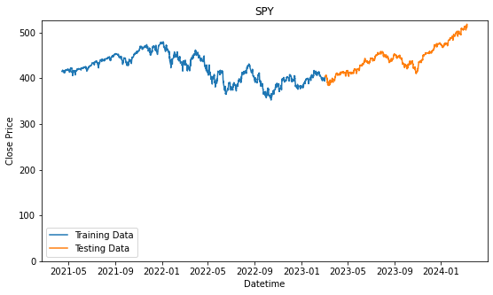
Therefore, we will be using these three stocks for the baseline strategies. Additionally, we will also be using the the SPDR S&P 500 ETF Trust (SPY), which is a stock that tracks the S&P 500 performance and at a lower price.
Limitations
Baseline Model Complexity
For the sake of simplicity for the comparison performed in this coursework, we will limit the scope by assuming that the investor will only be purchasing one type of stock for every given strategy. If we had given the option to hold more than 1, the complexity of the model increases. This is because not only will we need to optimize the purchasing and selling of the stock, we will then need to have some way to optimize the weightage and the choice of stock the investor would like to hold.
Inflationary factors, Tax and Fees
The following model comparisons will not take inflation into account, and also any other regulatory tax. Because trading fees or management fee of any kind is highly depending on what investment services an individual uses, we will not be including this into our model as well.
Buying only
Because investment and trading strategies can quickly scale in difficulty and the dimensions of data that can be used, etc, we will limit all the strategies to only buying a stock and selling the stock that are being held. While the market does allow short-selling, which is selling of a stock that one does not own, this would also further add another layer of complexity and dimension that we would need to consider.
Stars Aligned
As much as we are using data to trying substantiate our decisions and creating an investment strategy, there also could be the aspect of luck, where it just so happens that our analysis and strategy coincide with days of high performance, which might skew the data for having higher returns, or the opposite. Furthermore, because they are so many factors that affect the stock market, and we are only exploring one aspect of it, the analysis performed might show perfect or obvious expandability, but once again, it could just be because of coincidence and our analysis may not actually reflect what is happening in the stock market. While we are in the search for an edge in the market, it needs to be accepted that it will not be an easy tasks and simple analysis such as the following can truly give an edge. But we can explore and see if such analysis performed, are able to at least outperform is the simple strategies.
Getting the Data
Before we can test the performance of these baseline strategies, we will need to download and extract the data. Similarly, shown in coursework one, the fastest and easiest way to do so is by using the 'yfinance' library and extract it. But the drawback for this is that we do not have the freedom to get the specific characteristic data. For example, by have a 1hr interval dataset, where we can see hourly changes to the prices, we only can go as far back as 2 years. Only if we were to use daily prices, where the change in price only happens every day, we then can extract a longer timeframe.
The following code is used to get the data from Yahoo Finance using 'yfinance'. We have saved the data so that the rest of the coursework can be replicable. Hence, the following code is commented.
## This was initially used when we do not have the data
## Using yfinance get the a 730 day of 1 hour interval financial data

#stocks = {}
#stocks_list = ["PDD", "MDB", "DASH", "SPY"]

#for stock in stocks_list:

#    # Extracting the data for the chosen ticker, having about 2 years of data, in 1 hour interval
#    stocks[stock] = yf.Ticker(stock).history(period='730d', interval='1h')

#    # Saving these dataset so that it can results can be replicable
#    stocks[stock].to_csv("stock_data" + "\\" + stock)
The following code is to read the data that was downloaded using the code above. We will store the extracted data into a dictionary, with the index of the stock's ticker.
stocks = {}
stocks_list = ["PDD", "MDB", "DASH", "SPY"]

for stock in stocks_list:

    # Extract the downloaded data
    stocks[stock] = pd.read_csv("stock_data" + "\\" + stock)

stocks{'PDD': Datetime Open High Low \
0 2021-04-15 09:30:00-04:00 134.850006 134.919998 131.889999
1 2021-04-15 10:30:00-04:00 132.759995 132.860001 131.009995
2 2021-04-15 11:30:00-04:00 131.149994 132.000000 131.070007
3 2021-04-15 12:30:00-04:00 131.324997 132.000000 131.125000
4 2021-04-15 13:30:00-04:00 131.649994 132.600006 131.649994
... ... ... ... ...
5089 2024-03-08 11:30:00-05:00 110.870003 111.160004 108.870003
5090 2024-03-08 12:30:00-05:00 110.190002 111.139999 109.540001
5091 2024-03-08 13:30:00-05:00 111.099998 111.160004 110.510002
5092 2024-03-08 14:30:00-05:00 110.930000 111.209999 109.870003
5093 2024-03-08 15:30:00-05:00 110.230003 110.459999 109.919998
Close Volume Dividends Stock Splits
0 132.725006 646190 0.0 0.0
1 131.229904 481802 0.0 0.0
2 131.320007 246441 0.0 0.0
3 131.639999 252910 0.0 0.0
4 131.929993 354850 0.0 0.0
... ... ... ... ...
5089 110.160004 2595785 0.0 0.0
5090 111.099998 1317783 0.0 0.0
5091 110.910004 770590 0.0 0.0
5092 110.235001 1065732 0.0 0.0
5093 110.339996 1566768 0.0 0.0
[5094 rows x 8 columns],
'MDB': Datetime Open High Low \
0 2021-04-15 09:30:00-04:00 313.010010 317.940002 308.170013
1 2021-04-15 10:30:00-04:00 310.989990 314.670013 309.480011
2 2021-04-15 11:30:00-04:00 313.092987 318.929993 312.869995
3 2021-04-15 12:30:00-04:00 317.970001 317.970001 315.299988
4 2021-04-15 13:30:00-04:00 317.635010 321.470001 317.635010
... ... ... ... ...
5089 2024-03-08 11:30:00-05:00 381.329987 387.989899 381.000000
5090 2024-03-08 12:30:00-05:00 386.500000 388.000000 381.079987
5091 2024-03-08 13:30:00-05:00 384.119995 390.000000 381.559998
5092 2024-03-08 14:30:00-05:00 384.415009 389.464996 384.364990
5093 2024-03-08 15:30:00-05:00 385.475006 387.450012 383.184998
Close Volume Dividends Stock Splits
0 311.209991 92921 0.0 0.0
1 312.670013 55547 0.0 0.0
2 318.079987 81290 0.0 0.0
3 317.605011 56501 0.0 0.0
4 319.959991 88311 0.0 0.0
... ... ... ... ...
5089 386.524994 455519 0.0 0.0
5090 384.000000 483851 0.0 0.0
5091 384.359985 522412 0.0 0.0
5092 385.424988 480558 0.0 0.0
5093 383.420013 600317 0.0 0.0
[5094 rows x 8 columns],
'DASH': Datetime Open High Low \
0 2021-04-15 09:30:00-04:00 145.000000 152.449997 144.869995
1 2021-04-15 10:30:00-04:00 151.899994 154.880005 151.350006
2 2021-04-15 11:30:00-04:00 152.660004 153.270004 151.240005
3 2021-04-15 12:30:00-04:00 153.070007 154.169998 152.039993
4 2021-04-15 13:30:00-04:00 153.985001 154.500000 151.699997
... ... ... ... ...
5089 2024-03-08 11:30:00-05:00 131.850006 132.559998 131.429993
5090 2024-03-08 12:30:00-05:00 132.220001 132.220001 129.580002
5091 2024-03-08 13:30:00-05:00 129.649994 130.770004 129.309998
5092 2024-03-08 14:30:00-05:00 130.649994 131.779999 130.589996
5093 2024-03-08 15:30:00-05:00 131.259995 131.970001 131.130005
Close Volume Dividends Stock Splits
0 151.964996 693400 0.0 0.0
1 152.500000 802458 0.0 0.0
2 153.139999 287421 0.0 0.0
3 153.884995 360681 0.0 0.0
4 152.520004 285774 0.0 0.0
... ... ... ... ...
5089 132.149994 408198 0.0 0.0
5090 129.649994 630248 0.0 0.0
5091 130.639999 395151 0.0 0.0
5092 131.300003 467565 0.0 0.0
5093 131.800003 575430 0.0 0.0
[5094 rows x 8 columns],
'SPY': Datetime Open High Low \
0 2021-04-15 09:30:00-04:00 413.970001 414.559998 413.690002
1 2021-04-15 10:30:00-04:00 414.559998 415.459991 414.554993
2 2021-04-15 11:30:00-04:00 414.648987 415.230011 414.519989
3 2021-04-15 12:30:00-04:00 415.179993 415.700012 415.089996
4 2021-04-15 13:30:00-04:00 415.299011 415.670105 415.239990
... ... ... ... ...
5087 2024-03-08 11:30:00-05:00 514.750000 515.280029 513.570007
5088 2024-03-08 12:30:00-05:00 514.640015 514.840027 512.059998
5089 2024-03-08 13:30:00-05:00 512.440002 513.679993 511.130005
5090 2024-03-08 14:30:00-05:00 513.460022 514.460022 511.779999
5091 2024-03-08 15:30:00-05:00 511.929993 512.820007 511.720001
Close Volume Dividends Stock Splits Capital Gains
0 414.559998 11736294 0.0 0.0 0.0
1 414.645691 8902400 0.0 0.0 0.0
2 415.170013 5516651 0.0 0.0 0.0
3 415.290009 5138590 0.0 0.0 0.0
4 415.609985 5492613 0.0 0.0 0.0
... ... ... ... ... ...
5087 514.630005 11839572 0.0 0.0 0.0
5088 512.330017 10341053 0.0 0.0 0.0
5089 513.460022 10139821 0.0 0.0 0.0
5090 511.929993 9164240 0.0 0.0 0.0
5091 511.720001 9928936 0.0 0.0 0.0
[5092 rows x 9 columns]}Define a function to plot the stock
Define a function so that it will be easier for us to repeatedly plot when needed.
def plot_stock(stock):
    plt.figure(figsize=(10,5))

    df = stocks[stock].copy()
    df['Datetime'] = pd.to_datetime(df['Datetime'], errors='coerce', utc=True)
    df = df.set_index('Datetime')

    plt.plot(df['Close'])
    plt.gcf().autofmt_xdate()
    plt.xlabel('Datetime')
    plt.ylabel('Close Price')
    plt.title(stock)
    plt.show()
for stock in stocks_list:
plot_stock(stock)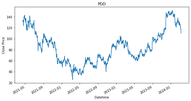
Creating DataFrame to store all performances
performances = pd.DataFrame(columns = ['Stock Ticker', 'Buy and Hold'])
performances['Stock Ticker'] = stocks_list
performances = performances.set_index('Stock Ticker')

performances
Buy and Hold
Stock Ticker
PDD NaN
MDB NaN
DASH NaN
SPY NaNBuy and Hold
There will be 4 outputs for this. The 3 stocks and the index fund.
For this strategy, it is a simple calculation will suffice. We will only need to take the percentage difference between the first row and the last row.
buy_and_hold_performances = []

for stock in stocks_list:

    print(stock)

    last_price = stocks[stock]['Close'].iloc[-1]
    cost_price = stocks[stock]['Open'].iloc[0]
    print("Last Price: ", last_price)
    print("Cost Price: ", cost_price)

    percent_return = (last_price - cost_price) / (cost_price)
    print("Return (%): ", percent_return * 100)

    buy_and_hold_performances.append(percent_return)

    print()

    plt.figure(figsize=(10,5))

    df = stocks[stock].copy()
    df['Datetime'] = pd.to_datetime(df['Datetime'], errors='coerce', utc=True)
    df = df.set_index('Datetime')

    plt.axhline(df.loc[df.index[0],'Close'],linestyle='--',color='g',label='Entry')
    plt.axhline(df.loc[df.index[-1],'Close'],linestyle='--',color='r',label='Final Price')
    plt.plot(df['Close'])

    plt.gcf().autofmt_xdate()
    plt.xlabel('Datetime')
    plt.ylabel('Close Price')
    plt.ylim(0)
    plt.title(stock)
    plt.legend()
    plt.show()

performances['Buy and Hold'] = buy_and_hold_performances
performances
PDD
Last Price: 110.33999633789062
Cost Price: 134.85000610351562
Return (%): -18.175757253440725
MDB
Last Price:  383.4200134277344
Cost Price:  313.010009765625
Return (%):  22.494489462120022
DASH
Last Price:  131.8000030517578
Cost Price:  145.0
Return (%):  -9.103446171201508
SPY
Last Price:  511.7200012207031
Cost Price:  413.9700012207031
Return (%):  23.612822115553676
              Buy and Hold
Stock Ticker
PDD              -0.181758
MDB               0.224945
DASH             -0.091034
SPY               0.236128
As shown in the results, there are stocks, such as PDD and DASH that have dropped in price from where it has started. This is indicated by the green line being above the red line. If the green line is above the red line, that means we have bought a stock above the final price, which will result in a loss. It is fine though as we still use it as a baseline, as we would like to find out if any other strategies can perform better than the loss that is produced by this baseline strategy. Will the other strategy produce a lower loss or will there be able to produce a profit.
Additionally, as shown, that given if an investor had invested during the start of the dataset, 15 April 2021, and held each of the stock until 8th March 2024, they would have ended up with a return/profit of the shown percentage in the performance DataFrame.
Dollar Cost Averaging
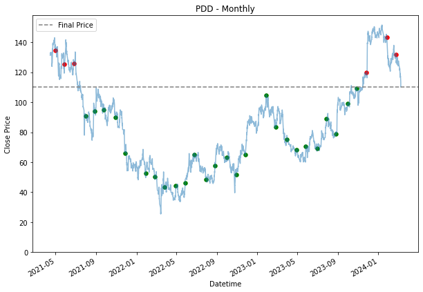
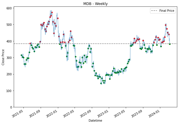
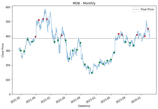
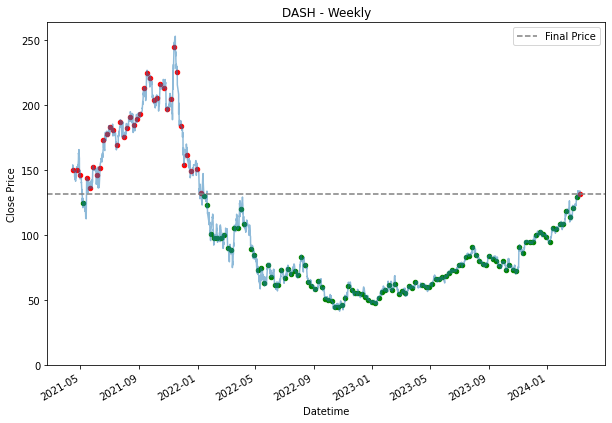
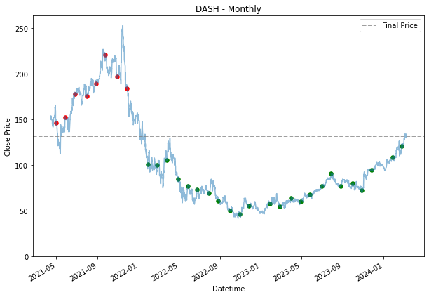
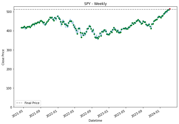
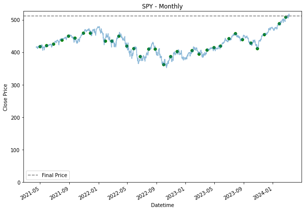
As for dollar cost averaging, the strategy is to go into the market at consistent and spread out pace, rather than entering all in one go. Spreading the starting fund throughout. Deciding on the frequency is also something that we can get into and properly optimize, as we can choose which day or time to buy, how frequent to buy like everyday or weekly or monthly, etc. Therefore, we will explore if we were to buy it daily, weekly and monthly. For weekly and monthly, we will go into the market on Friday, and for all of the frequency, we will enter at end of the day, so when the market is about to close.
for stock in stocks_list:

    df = stocks[stock].copy()
    df['Datetime'] = pd.to_datetime(df['Datetime'], errors='coerce', utc=True)
    last_price = stocks[stock]['Close'].iloc[-1]

    daily_dca = df[df['Datetime'].dt.hour == 15].copy()
    daily_dca['Return'] = daily_dca['Close'].map(lambda x: ((last_price - x) / x))
    performances.loc[stock, 'Dollar Cost Averaging (Daily)'] = daily_dca['Return'].sum() / len(daily_dca)

    plt.figure(figsize=(10,7))
    df = df.set_index('Datetime')
    plt.plot(df['Close'], alpha = 0.5)
    for entry in daily_dca['Datetime']:
        plt.scatter(entry, df.loc[entry, 'Close'],
                    color = 'g' if df.loc[entry, 'Close'] < df.loc[df.index[-1], 'Close'] else 'r',
                    s = 10
        )
    plt.axhline(df.loc[df.index[-1], 'Close'], color = 'grey', linestyle = '--', label= 'Final Price')
    plt.gcf().autofmt_xdate()
    plt.ylim(0)
    plt.xlabel('Datetime')
    plt.ylabel('Close Price')
    plt.title(stock)
    plt.legend()
    plt.show()

performances
              Buy and Hold  Dollar Cost Averaging (Daily)
Stock Ticker
PDD              -0.181758                       0.489227
MDB               0.224945                       0.254254
DASH             -0.091034                       0.552831
SPY               0.236128                       0.200805
Because a daily DCA means that an investor would be buying stock everyday. Hence, we see many dots appearing all over the chart. The grey line represent the final price at that we are using. Entries where it is below the line, are making money, and those that are above are losing money. Hence, it is why it is highlighted in green or red. Green for those that are below the line, which are making a profit, and those that are in red are losing money. the further away the dots are from the grey line, the more the entry is making or losing money.
Already, by using a daily dollar cost averaging, we see more returns for PDD and DASH. This is also because the price movement for PDD and DASH, is the exact scenario why an investor should DCA. When, the prices fall, you would want to pick up their share bit by bit, assuming it is a share an investor believes the prices will go up eventually and as shown for the SPY stock, where growth over time was steady, it was better to had held it from the start than to buy into it overtime. SPY is a good example of the downside of DCA.
for stock in stocks_list:

    df = stocks[stock].copy()
    df['Datetime'] = pd.to_datetime(df['Datetime'], errors='coerce', utc=True)
    last_price = stocks[stock]['Close'].iloc[-1]

    weekly_dca = df[(df['Datetime'].dt.hour == 15) & (df['Datetime'].dt.day_of_week == 4)].copy()
    weekly_dca['Return'] = weekly_dca['Close'].map(lambda x: ((last_price - x) / x))
    performances.loc[stock, 'Dollar Cost Averaging (Weekly)'] = weekly_dca['Return'].sum() / len(weekly_dca)

    plt.figure(figsize=(10,7))
    df = df.set_index('Datetime')

    plt.plot(df['Close'], alpha = 0.5)
    for entry in weekly_dca['Datetime']:

        plt.scatter(entry, df.loc[entry, 'Close'],
                    color = 'g' if df.loc[entry, 'Close'] < df.loc[df.index[-1], 'Close'] else 'r',
                    s = 20
        )

    plt.axhline(df.loc[df.index[-1], 'Close'], color = 'grey', linestyle = '--', label= 'Final Price')
    plt.gcf().autofmt_xdate()
    plt.ylim(0)
    plt.xlabel('Datetime')
    plt.ylabel('Close Price')
    plt.title(stock + ' - Weekly')
    plt.legend()
    plt.show()

    monthly_dca = weekly_dca.copy()
    monthly_dca['Month'] = monthly_dca['Datetime'].dt.month
    monthly_dca['Last Friday'] = monthly_dca['Month'].shift(-1) - monthly_dca['Month']
    monthly_dca = monthly_dca[monthly_dca['Last Friday'] == 1]
    monthly_dca['Return'] = monthly_dca['Close'].map(lambda x: ((last_price - x) / x))
    performances.loc[stock, 'Dollar Cost Averaging (Monthly)'] = monthly_dca['Return'].sum() / len(monthly_dca)

    plt.figure(figsize=(10,7))
    plt.plot(df['Close'], alpha = 0.5)
    for entry in monthly_dca['Datetime']:

        plt.scatter(entry, df.loc[entry, 'Close'],
                    color = 'g' if df.loc[entry, 'Close'] < df.loc[df.index[-1], 'Close'] else 'r',
                    s = 30
        )

    plt.axhline(df.loc[df.index[-1], 'Close'], color = 'grey', linestyle = '--', label= 'Final Price')
    plt.gcf().autofmt_xdate()
    plt.ylim(0)
    plt.xlabel('Datetime')
    plt.ylabel('Close Price')
    plt.title(stock + ' - Monthly')
    plt.legend()
    plt.show()

performances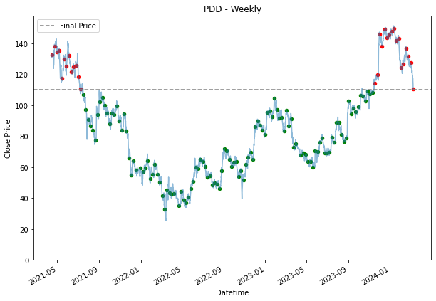
              Buy and Hold  Dollar Cost Averaging (Daily)  \
Stock Ticker
PDD              -0.181758                       0.489227
MDB               0.224945                       0.254254
DASH             -0.091034                       0.552831
SPY               0.236128                       0.200805

              Dollar Cost Averaging (Weekly)  Dollar Cost Averaging (Monthly)
Stock Ticker
PDD                                 0.472529                         0.503826
MDB                                 0.253272                         0.242322
DASH                                0.556192                         0.554912
SPY                                 0.200736                         0.200701
for stock in stocks_list:
df = stocks[stock].copy()
df['Datetime'] = pd.to_datetime(df['Datetime'], errors='coerce', utc=True)
last_price = stocks[stock]['Close'].iloc[-1]
hourly_dca = df.copy()
hourly_dca['Return'] = hourly_dca['Close'].map(lambda x: ((last_price - x)/ x))
performances.loc[stock, 'Dollar Cost Averaging (Hourly)'] = hourly_dca['Return'].sum() / len(hourly_dca)
performances Buy and Hold Dollar Cost Averaging (Daily) \
Stock Ticker
PDD -0.181758 0.489227
MDB 0.224945 0.254254
DASH -0.091034 0.552831
SPY 0.236128 0.200805
Dollar Cost Averaging (Weekly) Dollar Cost Averaging (Monthly) \
Stock Ticker
PDD 0.472529 0.503826
MDB 0.253272 0.242322
DASH 0.556192 0.554912
SPY 0.200736 0.200701
Dollar Cost Averaging (Hourly)
Stock Ticker
PDD 0.490052
MDB 0.254119
DASH 0.552687
SPY 0.200839Similarly, the same visualization technique is used to demonstrate the 'buy and hold' strategy, was not created for the hourly one because it would be mess as there are going to be so many entries.
Based on the performance collected, in most cases, it outperformed the 'buy and hold' strategy, but it is not as effective for the SPY. Because of the steadier uptrend, DCA is not as effective. As for MDB, we can see that it is quite a volatile stock and due to this volatility, we can see that there are about equal amounts of green there is as to red. In a situation like this, neither baseline strategies are getting an edge.
Using Traditional Data Analysis
In this part, we will be using the some simple data analysis such as finding the day that has the most positive price movement, is there any particular hour that results in the most price movement, etc. By exploring these trend, we will try to see if we can create any strategies that could beat the baseline strategies above.
One thing to note is that, for the strategies above, we did not really need to bother about the exit of any of the purchase of stock. Exit, as in selling a purchased stock, or closing the position. Only by doing so, we are able to have realized profits or losses. On the other hand, the strategies below, will need to take that into account.
Limitation
Length of Time for Investing
Using this method, similar to how we train a machine learning model, we will need have a training set and a test set. Because, we need some data to validate if the strategy works. This might benefit the strategy because it is exposed to the market for lesser duration, but it could work against it where the strategy does not have enough time to accumulate and realize any positive price movement. Therefore, given that there are 730 days of 1 hour data, which is around 5094 rows of data and we will use 475 days as training data, which will be around 3311 rows of data, where we will use it to identify trends and patterns, and then test it out with the remaining days to see if we are able beat the strategies above.
The use of percentage change - 1 hour rate
Because by using the percentage change, it gives more meaningful data to the actual price movement, we can have a better comparison with across the different stocks. However, the downside of preprocessing price this way is that we are locked into the the 1 hour rate and the strategy might need to revolve around by the fact. For example, if we were to find which hour will give us the best average return, we have to get into the market at that hour, and then exit it immediately
The limitation stated in the above, section also applies to this as well.
Findings from Coursework 1
In coursework 1, used percentage change between the hours to find out the average pattern that could lead to a high percentage return in the next hour. We also explored that by extracting the date time information, we can find simple trends such as the average return of a given day at which hour.
Therefore, we will be re-doing the findings from coursework 1, but with only 475 days of data, then, we will put it to the test and see if we are able to use the decisions made using our data analysis to make investment decisions.
Pre-process Data
We will also need to create a column for the percentage return. We will use the next row's close price, to determine what is the percentage change of the current row. So that we know that if we were to invest at this hour, what is the next amount of percentage change can we expect.
Then, we will then need to also extract the date time features, so that we can use it to find trends and pattern. and finally split it into training data and testing data. Most of these steps are already shown in coursework 1.
training_stock_data = {}
testing_stock_data = {}

for stock in stocks_list:

    # Referencing the value the stock DataFrame
    df = stocks[stock].copy()

    # By using shift(-1), we can access the close price of the next row
    df['% Change in Close Price'] = (df['Close'].shift(-1) - df['Close']) / df['Close']

    # Extracting the datetime feature
    df['Datetime'] = pd.to_datetime(df['Datetime'],errors='coerce',utc=True)
    df['Datetime'] = df['Datetime'].dt.tz_localize(None)
    df['Hour'] = df['Datetime'].dt.hour
    df['Day'] = df['Datetime'].dt.day
    df['Day_of_Week'] = df['Datetime'].dt.day_of_week
    df['Month'] = df['Datetime'].dt.month

    min_hour = df['Hour'].min()
    df['Hour'] = df['Hour'] - min_hour

    # Splitting it into training and splitting. 65% training and 35% testing
    training_stock_data[stock] = df[:3312]
    testing_stock_data[stock] = df[3312:-1]

training_stock_data['DASH'].head()
Datetime Open High Low Close Volume \
0 2021-04-15 13:30:00 145.000000 152.449997 144.869995 151.964996 693400
1 2021-04-15 14:30:00 151.899994 154.880005 151.350006 152.500000 802458
2 2021-04-15 15:30:00 152.660004 153.270004 151.240005 153.139999 287421
3 2021-04-15 16:30:00 153.070007 154.169998 152.039993 153.884995 360681
4 2021-04-15 17:30:00 153.985001 154.500000 151.699997 152.520004 285774
Dividends Stock Splits % Change in Close Price Hour Day Day_of_Week \
0 0.0 0.0 0.003521 0 15 3
1 0.0 0.0 0.004197 1 15 3
2 0.0 0.0 0.004865 2 15 3
3 0.0 0.0 -0.008870 3 15 3
4 0.0 0.0 -0.010556 4 15 3
Month
0 4
1 4
2 4
3 4
4 4for stock in stocks_list:
plt.figure(figsize=(9,5))
df = training_stock_data[stock].copy()
df2 = testing_stock_data[stock].copy()
df = df.set_index('Datetime')
df2 = df2.set_index('Datetime')
plt.plot(df['Close'],label='Training Data')
plt.plot(df2['Close'], label='Testing Data')
plt.xlabel('Datetime')
plt.ylabel('Close Price')
plt.title(stock)
plt.legend()
plt.ylim(0)
plt.show()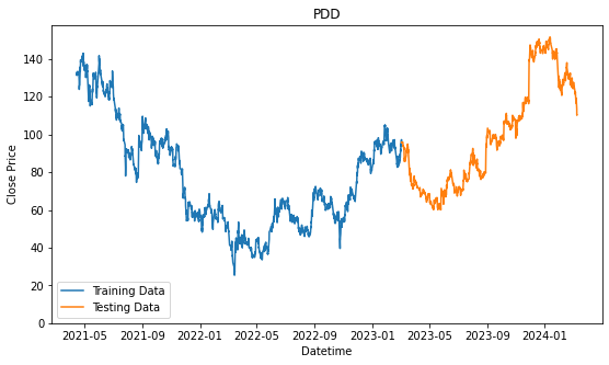
We will prepare another one where we consolidated all the stocks selected into one. By analyzing all of them together, we might find a better pattern because we have the more data to validate the pattern or trend. On the other hand, it might give us worst performance because of how general the patterns that are identified and it may not be specifically applicable to the individual stock.
consolidated_training_stock_data = pd.DataFrame()

for stock in stocks_list:
    consolidated_training_stock_data = pd.concat([training_stock_data[stock], consolidated_training_stock_data],
                                                 ignore_index= True, sort = False)
Data Analysis
We will be using the training stock data and the consolidated stock data, to find some trends and patterns, and then test it to see its performance. Unlike 'buy and hold' and 'dollar cost averaging', for the return calculation for the following strategies purpose, we will not only be entering the market according to our analysis, but also exiting the market (selling our position, or selling the position we have) because of how we have changed processed the absolute price to percentage change, by the hour.
Best Hour Every Day
We will start of by finding what is the best hour to have a one hour trade. Then, we will test out what kind of performance are can we expect from using this strategy.
Individual Stock
average_return_hourly_individual = pd.DataFrame(columns=['Stock', 'Hour', '% Change in Close Price'])

for stock in stocks_list:

    print(stock)
    df = training_stock_data[stock].copy()

    min_hour = df['Hour'].min()
    max_hour = df['Hour'].max()

    for hour in range(min_hour,max_hour+1):

        temp = df.loc[(df['Hour'] == hour),'% Change in Close Price'].mean()
        average_return_hourly_individual.loc[len(average_return_hourly_individual.index)] = \
            [stock, hour-min_hour, temp]

        print(
            'The average return on the hour ' + str(hour) + '\t' +
            "{:.3f}".format(temp * 100) + '%'
        )

    print()

average_return_hourly_individual_top3 = average_return_hourly_individual.sort_values(['Stock','% Change in Close Price'],ascending=False)\
    .groupby('Stock').head(3)

average_return_hourly_individual_top3
PDD
The average return on the hour 0 -0.140%
The average return on the hour 1 0.010%
The average return on the hour 2 -0.073%
The average return on the hour 3 0.056%
The average return on the hour 4 0.040%
The average return on the hour 5 0.010%
The average return on the hour 6 0.166%
The average return on the hour 7 -0.063%
MDB
The average return on the hour 0 -0.102%
The average return on the hour 1 -0.064%
The average return on the hour 2 -0.037%
The average return on the hour 3 0.005%
The average return on the hour 4 0.100%
The average return on the hour 5 -0.011%
The average return on the hour 6 0.093%
The average return on the hour 7 0.064%
DASH
The average return on the hour 0 0.028%
The average return on the hour 1 -0.133%
The average return on the hour 2 -0.078%
The average return on the hour 3 -0.028%
The average return on the hour 4 0.072%
The average return on the hour 5 0.009%
The average return on the hour 6 0.039%
The average return on the hour 7 0.023%
SPY
The average return on the hour 0 0.004%
The average return on the hour 1 -0.015%
The average return on the hour 2 -0.004%
The average return on the hour 3 0.003%
The average return on the hour 4 0.028%
The average return on the hour 5 -0.001%
The average return on the hour 6 -0.003%
The average return on the hour 7 -0.027%
   Stock  Hour  % Change in Close Price
28   SPY     4                 0.000279
24   SPY     0                 0.000039
27   SPY     3                 0.000031
6    PDD     6                 0.001662
3    PDD     3                 0.000559
4    PDD     4                 0.000396
12   MDB     4                 0.001002
14   MDB     6                 0.000925
15   MDB     7                 0.000643
20  DASH     4                 0.000725
22  DASH     6                 0.000394
16  DASH     0                 0.000285
Consolidated
average_return_hourly_consolidated = pd.DataFrame(columns=['Hour', '% Change in Close Price'])

df = consolidated_training_stock_data.copy()

min_hour = df['Hour'].min()
max_hour = df['Hour'].max()

for hour in range(min_hour,max_hour+1):

    temp = df.loc[(df['Hour'] == hour),'% Change in Close Price'].mean()
    average_return_hourly_consolidated.loc[len(average_return_hourly_consolidated.index)] = \
        [hour-min_hour, temp]

    print(
        'The average return on the hour ' + str(hour) + '\t' +
        "{:.3f}".format(temp*100) + '%'
    )

print()

average_return_hourly_consolidated.sort_values(['% Change in Close Price'],ascending=False)
The average return on the hour 0 -0.053%
The average return on the hour 1 -0.050%
The average return on the hour 2 -0.048%
The average return on the hour 3 0.009%
The average return on the hour 4 0.060%
The average return on the hour 5 0.002%
The average return on the hour 6 0.074%
The average return on the hour 7 -0.001%
   Hour  % Change in Close Price
6   6.0                 0.000738
4   4.0                 0.000600
3   3.0                 0.000088
5   5.0                 0.000017
7   7.0                -0.000009
2   2.0                -0.000481
1   1.0                -0.000504
0 0.0 -0.000525plt.figure(figsize=(13,7))
for stock in stocks_list:
temp = average_return_hourly_individual.loc[(average_return_hourly_individual['Stock'] == stock)].copy()
plt.plot(temp['Hour'],temp['% Change in Close Price'],label=stock,alpha=0.6)
plt.scatter(temp['Hour'],temp['% Change in Close Price'],alpha=0.6)
plt.plot(average_return_hourly_consolidated['Hour'],
average_return_hourly_consolidated['% Change in Close Price'],
label = 'Consolidated', linestyle = '--', linewidth = 5)
plt.legend()
plt.title("Average Hourly Return")
plt.xlabel('Hour')
plt.ylabel('% Change in Close Price')
plt.show()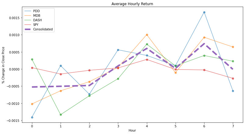
Based on our findings and results above, it seems that at hour 4 and 6, is where generally all of the stock from our small sample list, will have the biggest positive price movement. We will now proceed to use the testing set of data, to see what are the performances we are able to achieve.
The return column created here is to track, how much have we made or loss. Therefore, the column acts as a balance indicator, like in a bank account, and reflect the current return of a given row. Therefore, the final value in the column, should indicate the value we would want to see. Because the column is already in decimal, we can now just add 1 to the current percentage change in close price, and multiple by the previous result, which gives us the new current return at the given row.
General Best 3 Hours
Using the best three performing hours, derived from the consolidated list, this will be the strategy. We will purchase the stock according to the general best performing hours found with the consolidated list. Therefore, that would at hour 0, hour 4 and hour 6. The strategy is to buy in at the hour, and then sell the stock an hour later.
print("Using Training Data")
print("_____________________")

for stock in stocks_list:
    print(stock)
    df = training_stock_data[stock].copy()
    df['Datetime'] = pd.to_datetime(df['Datetime'], errors='coerce', utc=True)
    temp = df[(df['Hour'] == 4 ) | (df['Hour'] == 6) | (df['Hour'] == 3)].copy()

    temp['Returns'] = 0
    return_col = temp.columns.get_loc('Returns')
    change_in_close_price_col = temp.columns.get_loc('% Change in Close Price')

    for i in range(0, len(temp)):

        if i == 0:
            temp.iloc[i, return_col] = (1 + temp.iloc[i,change_in_close_price_col]) * 1
        else:
            temp.iloc[i, return_col] = (1 + temp.iloc[i,change_in_close_price_col]) * temp.iloc[i-1,return_col]

    performances.loc[stock, 'General Best 3 Hours - Training'] = temp.iloc[-1,return_col] - 1
    print(temp.iloc[-1,return_col])

    plt.figure(figsize=(15,9))

    df = df.set_index('Datetime')
    temp = temp.set_index('Datetime')

    plt.plot(df['Close'], alpha = 0.5)

    for entry in temp.index:

        plt.scatter(entry, df.loc[entry, 'Close'],
            color = 'g' if temp.loc[entry, '% Change in Close Price'] >= 0 else 'r',
            s = 10
        )

    plt.gcf().autofmt_xdate()
    plt.ylim(0)
    plt.xlabel('Datetime')
    plt.ylabel('Close Price')
    plt.title(stock + ' - Training')
    plt.show()

print("\n")
print("Using Testing Data")
print("_____________________")

for stock in stocks_list:
    print(stock)

    df = testing_stock_data[stock].copy()
    temp = df[(df['Hour'] == 4 ) | (df['Hour'] == 6) | (df['Hour'] == 3)].copy()

    temp['Returns'] = 0
    return_col = temp.columns.get_loc('Returns')
    change_in_close_price_col = temp.columns.get_loc('% Change in Close Price')

    for i in range(0, len(temp)):

        if i == 0:
            temp.iloc[i, return_col] = (1 + temp.iloc[i,change_in_close_price_col]) * 1
        else:
            temp.iloc[i, return_col] = (1 + temp.iloc[i,change_in_close_price_col]) * temp.iloc[i-1,return_col]

    performances.loc[stock, 'General Best 3 Hours - Testing'] = temp.iloc[-1,return_col] - 1
    print(temp.iloc[-1,return_col])

    plt.figure(figsize=(15,9))

    df = df.set_index('Datetime')
    temp = temp.set_index('Datetime')

    plt.plot(df['Close'], alpha = 0.5)

    for entry in temp.index:

        plt.scatter(entry, df.loc[entry, 'Close'],
            color = 'g' if temp.loc[entry, '% Change in Close Price'] >= 0 else 'r',
            s = 10
        )

    plt.gcf().autofmt_xdate()
    plt.ylim(0)
    plt.xlabel('Datetime')
    plt.ylabel('Close Price')
    plt.title(stock + ' - Testing')
    plt.show()

performances
Using Training Data
_____________________
PDD
2.1043466734327567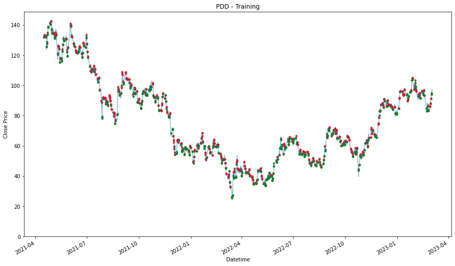
MDB
1.9001580234012414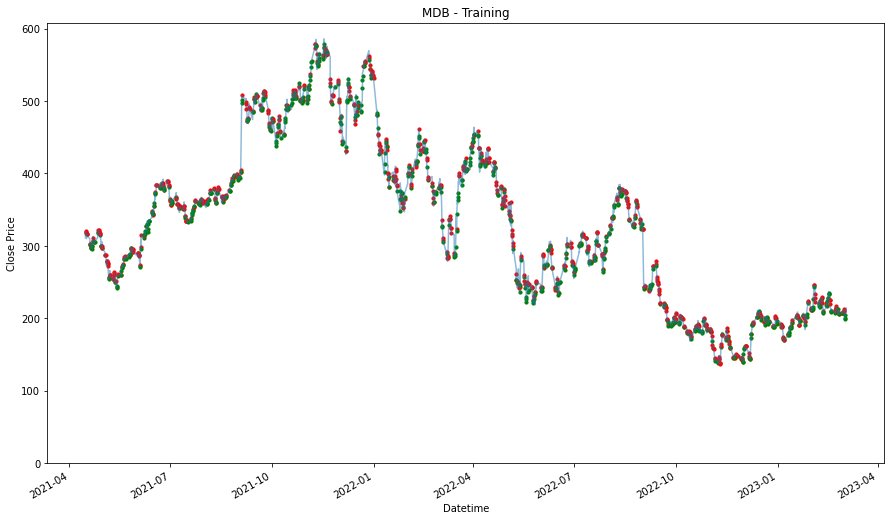
DASH
1.1354003896621916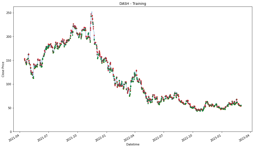
SPY
1.1216981139228874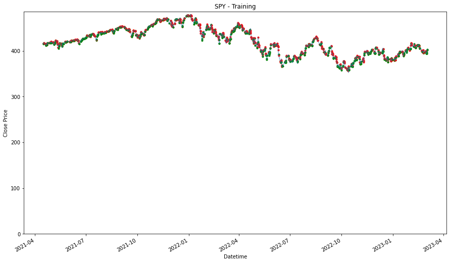
Using Testing Data
_____________________
PDD
0.8996901198051401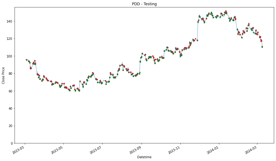
MDB
1.3587372122741483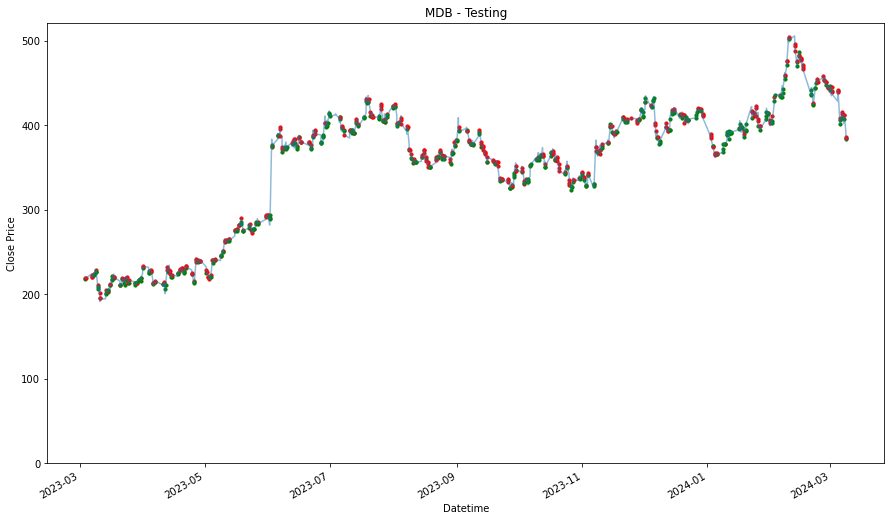
DASH
1.4780411991174967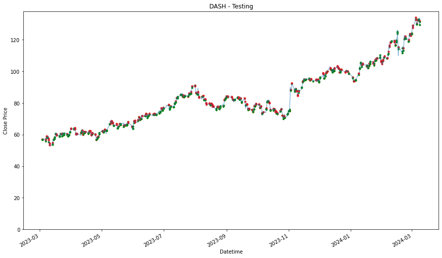
SPY
1.1229863011156784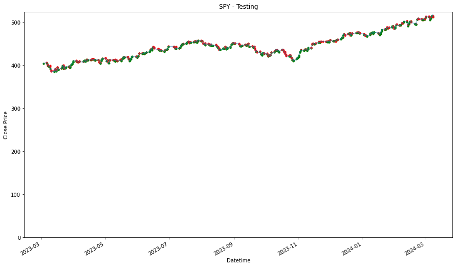
              Buy and Hold  Dollar Cost Averaging (Daily)  \
Stock Ticker
PDD              -0.181758                       0.489227
MDB               0.224945                       0.254254
DASH             -0.091034                       0.552831
SPY               0.236128                       0.200805

              Dollar Cost Averaging (Weekly)  Dollar Cost Averaging (Monthly)  \
Stock Ticker
PDD                                 0.472529                         0.503826
MDB                                 0.253272                         0.242322
DASH                                0.556192                         0.554912
SPY                                 0.200736                         0.200701

              Dollar Cost Averaging (Hourly)  General Best 3 Hours - Training  \
Stock Ticker
PDD                                 0.490052                         1.104347
MDB                                 0.254119                         0.900158
DASH                                0.552687                         0.135400
SPY                                 0.200839                         0.121698

              General Best 3 Hours - Testing
Stock Ticker
PDD                                -0.100310
MDB                                 0.358737
DASH                                0.478041
SPY                                 0.122986
General Best Hour
Using the best performing hour, derived from the consolidated list, this will be the strategy. We will purchase the stock according to the general best performing hour found with the consolidated list. Therefore, that would at hour 0, hour 4 and hour 6. The strategy is to buy in at the hour, and then sell the stock an hour later.
print("Using Training Data")
print("_____________________")

for stock in stocks_list:
    print(stock)

    df = training_stock_data[stock].copy()
    temp = df[(df['Hour'] == 6)].copy()

    temp['Returns'] = 0
    return_col = temp.columns.get_loc('Returns')
    change_in_close_price_col = temp.columns.get_loc('% Change in Close Price')

    for i in range(0, len(temp)):

        if i == 0:
            temp.iloc[i, return_col] = (1 + temp.iloc[i,change_in_close_price_col]) * 1
        else:
            temp.iloc[i, return_col] = (1 + temp.iloc[i,change_in_close_price_col]) * temp.iloc[i-1,return_col]

    performances.loc[stock, 'General Best Hour - Training'] = temp.iloc[-1,return_col] - 1
    print(temp.iloc[-1,return_col])


    plt.figure(figsize=(15,9))

    df = df.set_index('Datetime')
    temp = temp.set_index('Datetime')

    plt.plot(df['Close'], alpha = 0.5)

    for entry in temp.index:

        plt.scatter(entry, df.loc[entry, 'Close'],
            color = 'g' if temp.loc[entry, '% Change in Close Price'] >= 0 else 'r',
            s = 10
        )

    plt.gcf().autofmt_xdate()
    plt.ylim(0)
    plt.xlabel('Datetime')
    plt.ylabel('Close Price')
    plt.title(stock + ' - Training')
    plt.show()


print("\n")
print("Using Testing Data")
print("_____________________")

for stock in stocks_list:
    print(stock)

    df = testing_stock_data[stock].copy()
    temp = df[(df['Hour'] == 6)].copy()

    temp['Returns'] = 0
    return_col = temp.columns.get_loc('Returns')
    change_in_close_price_col = temp.columns.get_loc('% Change in Close Price')

    for i in range(0, len(temp)):

        if i == 0:
            temp.iloc[i, return_col] = (1 + temp.iloc[i,change_in_close_price_col]) * 1
        else:
            temp.iloc[i, return_col] = (1 + temp.iloc[i,change_in_close_price_col]) * temp.iloc[i-1,return_col]

    performances.loc[stock, 'General Best Hour - Testing'] = temp.iloc[-1,return_col] - 1
    print(temp.iloc[-1,return_col])

    plt.figure(figsize=(15,9))

    df = df.set_index('Datetime')
    temp = temp.set_index('Datetime')

    plt.plot(df['Close'], alpha = 0.5)

    for entry in temp.index:

        plt.scatter(entry, df.loc[entry, 'Close'],
            color = 'g' if temp.loc[entry, '% Change in Close Price'] >= 0 else 'r',
            s = 10
        )

    plt.gcf().autofmt_xdate()
    plt.ylim(0)
    plt.xlabel('Datetime')
    plt.ylabel('Close Price')
    plt.title(stock + ' - Testing')
    plt.show()

performances
Using Training Data
_____________________
PDD
1.3897785667065108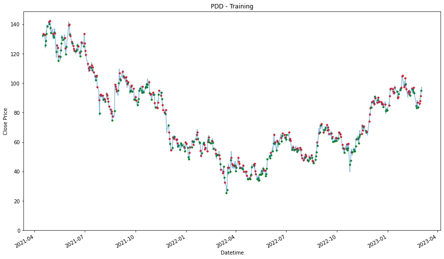
MDB
1.2144736634274178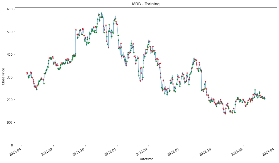
DASH
0.9756114959627441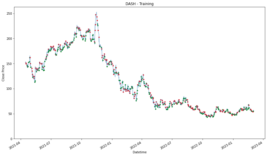
SPY
0.9742121489329175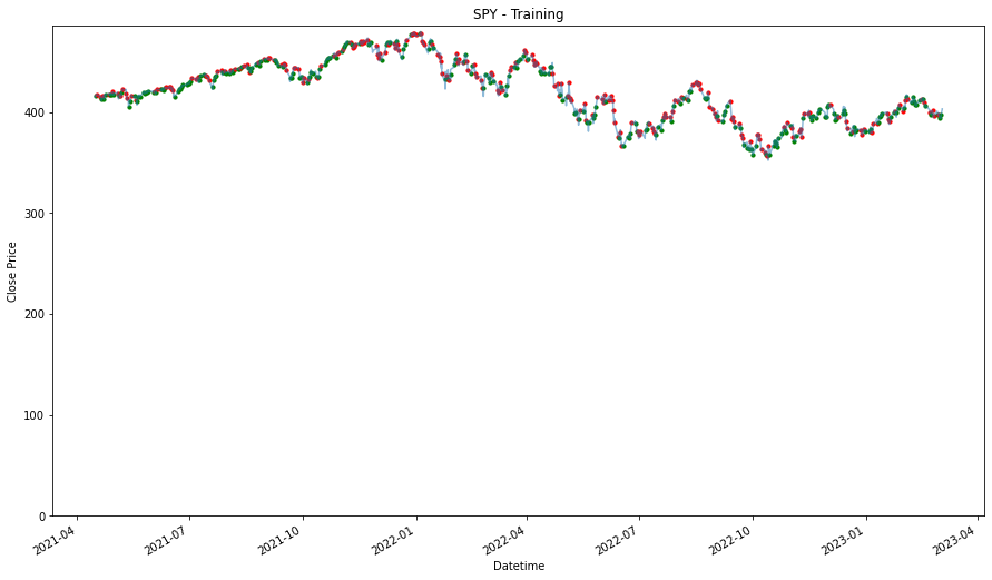
Using Testing Data
_____________________
PDD
0.962917971772168
MDB
1.5430558320874295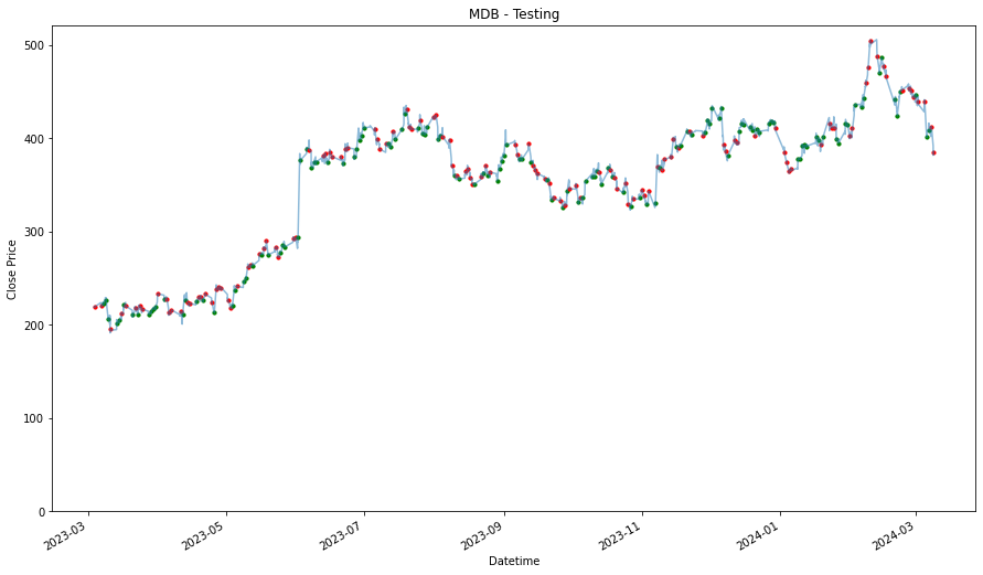
DASH
1.4687324315599015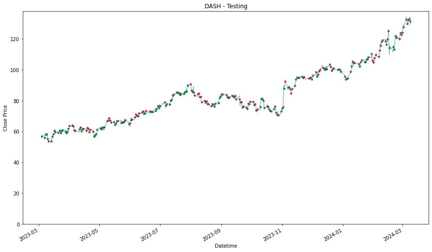
SPY
1.102683690578897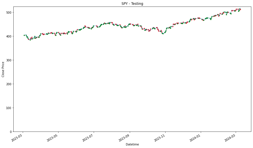
              Buy and Hold  Dollar Cost Averaging (Daily)  \
Stock Ticker
PDD              -0.181758                       0.489227
MDB               0.224945                       0.254254
DASH             -0.091034                       0.552831
SPY               0.236128                       0.200805

              Dollar Cost Averaging (Weekly)  Dollar Cost Averaging (Monthly)  \
Stock Ticker
PDD                                 0.472529                         0.503826
MDB                                 0.253272                         0.242322
DASH                                0.556192                         0.554912
SPY                                 0.200736                         0.200701

              Dollar Cost Averaging (Hourly)  General Best 3 Hours - Training  \
Stock Ticker
PDD                                 0.490052                         1.104347
MDB                                 0.254119                         0.900158
DASH                                0.552687                         0.135400
SPY                                 0.200839                         0.121698

              General Best 3 Hours - Testing  General Best Hour - Training  \
Stock Ticker
PDD                                -0.100310                      0.389779
MDB                                 0.358737                      0.214474
DASH                                0.478041                     -0.024389
SPY                                 0.122986                     -0.025788

              General Best Hour - Testing
Stock Ticker
PDD                             -0.037082
MDB                              0.543056
DASH                             0.468732
SPY                              0.102684
Individual Best 3 Hours
Because we have also analyzed them individually, we will try to use the individual best hours and also see the results.
individual_best_hour = {
    'SPY': [4,0,3],
    'PDD': [6,3,4],
    'MDB': [4,6,7],
    'DASH': [4,6,0]
}

print("Using Training Data")
print("_____________________")

for stock in stocks_list:
    print(stock)

    df = training_stock_data[stock].copy()
    temp = pd.DataFrame(columns = df.columns)

    for hour_no, best_hour in enumerate(individual_best_hour[stock]):

        if hour_no == 0:
            temp = df[(df['Hour'] == best_hour)]
        else:
            temp = pd.concat([temp, df[df['Hour'] == best_hour]])

    temp['Returns'] = 0
    return_col = temp.columns.get_loc('Returns')
    change_in_close_price_col = temp.columns.get_loc('% Change in Close Price')

    for i in range(0, len(temp)):
        if i == 0:
            temp.iloc[i, return_col] = (1 + temp.iloc[i,change_in_close_price_col]) * 1
        else:
            temp.iloc[i, return_col] = (1 + temp.iloc[i,change_in_close_price_col]) * temp.iloc[i-1,return_col]

    performances.loc[stock, 'Individual Best 3 Hours - Training'] = temp.iloc[-1,return_col] - 1
    print(temp.iloc[-1,return_col])

    plt.figure(figsize=(15,9))

    df = df.set_index('Datetime')
    temp = temp.set_index('Datetime')

    plt.plot(df['Close'], alpha = 0.5)

    for entry in temp.index:

        plt.scatter(entry, df.loc[entry, 'Close'],
            color = 'g' if temp.loc[entry, '% Change in Close Price'] >= 0 else 'r',
            s = 10
        )

    plt.gcf().autofmt_xdate()
    plt.ylim(0)
    plt.xlabel('Datetime')
    plt.ylabel('Close Price')
    plt.title(stock + ' - Training')
    plt.show()

print("\n")
print("Using Testing Data")
print("_____________________")

for stock in stocks_list:
    print(stock)

    df = testing_stock_data[stock].copy()
    temp = pd.DataFrame(columns = df.columns)

    for hour_no, best_hour in enumerate(individual_best_hour[stock]):

        if hour_no == 0:
            temp = df[(df['Hour'] == best_hour)]
        else:
            temp = pd.concat([temp, df[df['Hour'] == best_hour]])

    temp['Returns'] = 0
    return_col = temp.columns.get_loc('Returns')
    change_in_close_price_col = temp.columns.get_loc('% Change in Close Price')

    for i in range(0, len(temp)):
        if i == 0:
            temp.iloc[i, return_col] = (1 + temp.iloc[i,change_in_close_price_col]) * 1
        else:
            temp.iloc[i, return_col] = (1 + temp.iloc[i,change_in_close_price_col]) * temp.iloc[i-1,return_col]

    performances.loc[stock, 'Individual Best 3 Hours - Testing'] = temp.iloc[-1,return_col] - 1
    print(temp.iloc[-1,return_col])

    plt.figure(figsize=(15,9))

    df = df.set_index('Datetime')
    temp = temp.set_index('Datetime')

    plt.plot(df['Close'], alpha = 0.5)

    for entry in temp.index:

        plt.scatter(entry, df.loc[entry, 'Close'],
            color = 'g' if temp.loc[entry, '% Change in Close Price'] >= 0 else 'r',
            s = 10
        )

    plt.gcf().autofmt_xdate()
    plt.ylim(0)
    plt.xlabel('Datetime')
    plt.ylabel('Close Price')
    plt.title(stock + ' - Testing')
    plt.show()

performances.T
Using Training Data
_____________________
PDD
2.104346673432768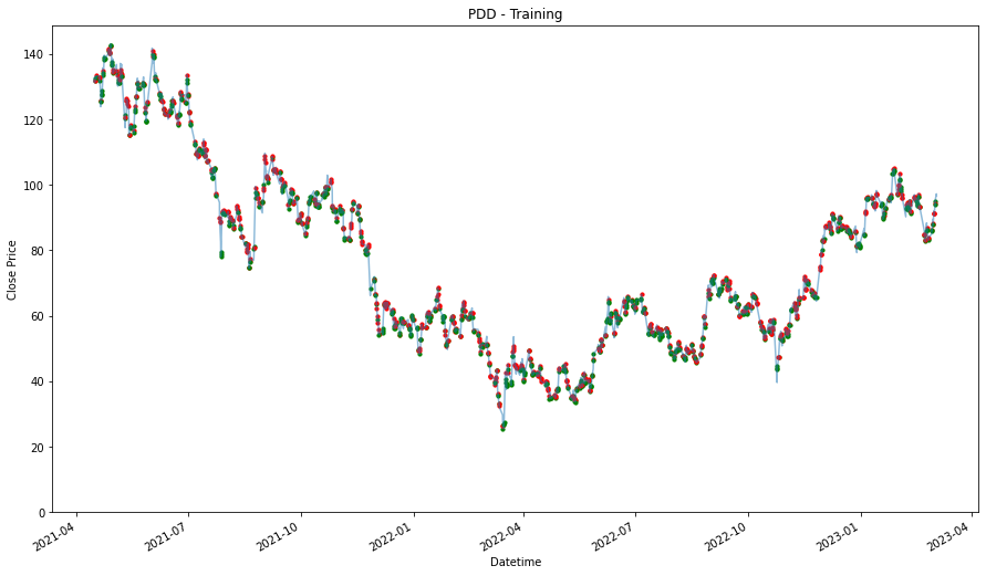
MDB
1.8456429990147925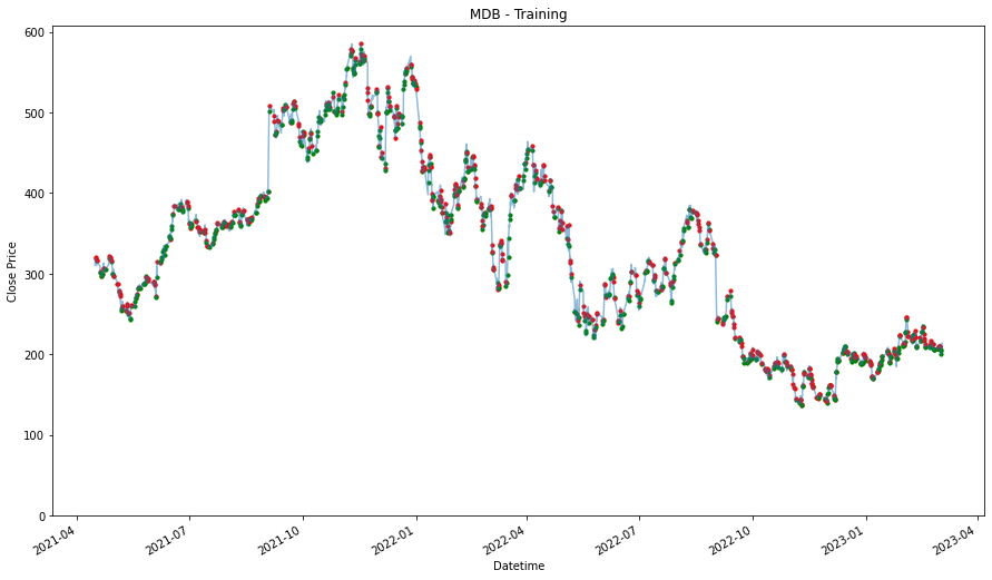
DASH
1.3813326734304454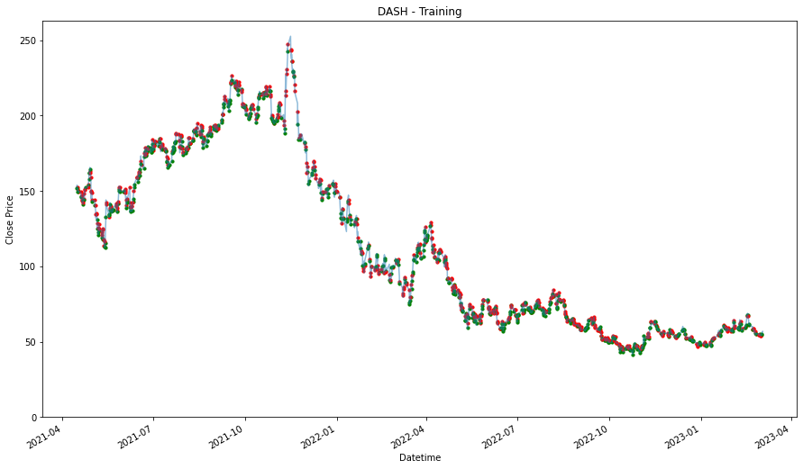
SPY
1.162690677935936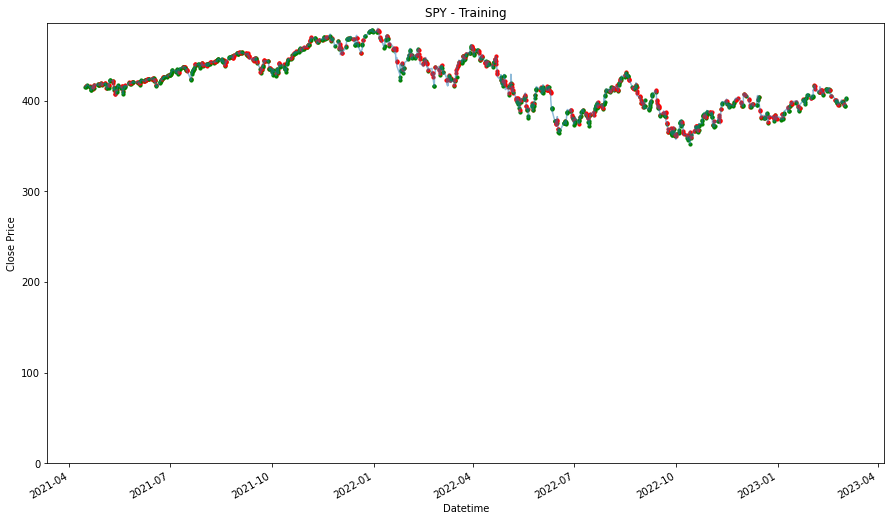
Using Testing Data
_____________________
PDD
0.899690119805139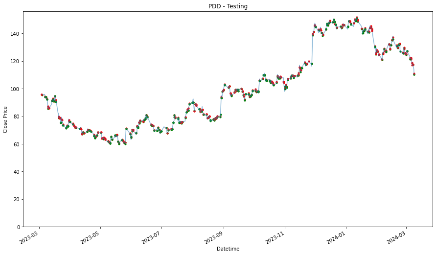
MDB
1.5007797791650734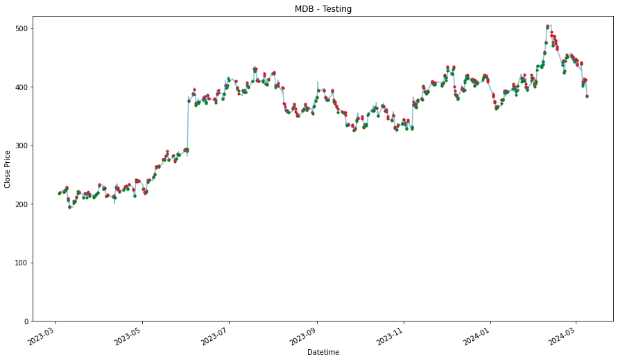
DASH
1.6466367874031884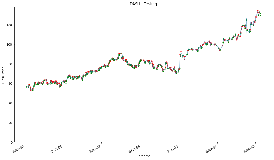
SPY
1.050682044985406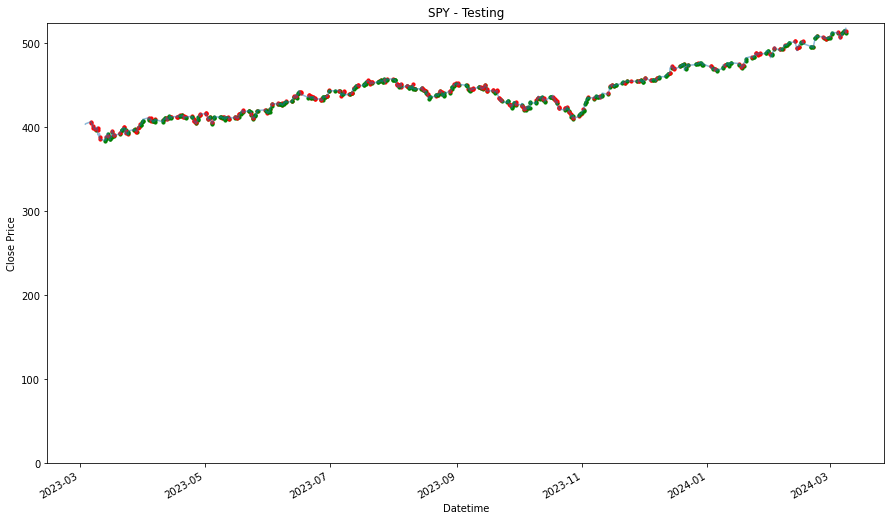
Stock Ticker                             PDD       MDB      DASH       SPY
Buy and Hold                       -0.181758  0.224945 -0.091034  0.236128
Dollar Cost Averaging (Daily)       0.489227  0.254254  0.552831  0.200805
Dollar Cost Averaging (Weekly)      0.472529  0.253272  0.556192  0.200736
Dollar Cost Averaging (Monthly)     0.503826  0.242322  0.554912  0.200701
Dollar Cost Averaging (Hourly)      0.490052  0.254119  0.552687  0.200839
General Best 3 Hours - Training     1.104347  0.900158  0.135400  0.121698
General Best 3 Hours - Testing     -0.100310  0.358737  0.478041  0.122986
General Best Hour - Training        0.389779  0.214474 -0.024389 -0.025788
General Best Hour - Testing        -0.037082  0.543056  0.468732  0.102684
Individual Best 3 Hours - Training  1.104347  0.845643  0.381333  0.162691
Individual Best 3 Hours - Testing  -0.100310  0.500780  0.646637  0.050682
Individual Best Hour
Now for the individual's best hours. The best hours are already arranged in the individual best hour. The first value in the list is the best hour.
print("Using Training Data")
print("_____________________")

for stock in stocks_list:
    print(stock)

    df = training_stock_data[stock].copy()
    temp = df[df['Hour']==individual_best_hour[stock][0]].copy()

    temp['Returns'] = 0
    return_col = temp.columns.get_loc('Returns')
    change_in_close_price_col = temp.columns.get_loc('% Change in Close Price')

    for i in range(0, len(temp)):
        if i == 0:
            temp.iloc[i, return_col] = (1 + temp.iloc[i,change_in_close_price_col]) * 1
        else:
            temp.iloc[i, return_col] = (1 + temp.iloc[i,change_in_close_price_col]) * temp.iloc[i-1,return_col]

    performances.loc[stock, 'Individual Best Hour - Training'] = temp.iloc[-1,return_col] - 1
    print(temp.iloc[-1,return_col])

    plt.figure(figsize=(15,9))

    df = df.set_index('Datetime')
    temp = temp.set_index('Datetime')

    plt.plot(df['Close'], alpha = 0.5)

    for entry in temp.index:

        plt.scatter(entry, df.loc[entry, 'Close'],
            color = 'g' if temp.loc[entry, '% Change in Close Price'] >= 0 else 'r',
            s = 10
        )

    plt.gcf().autofmt_xdate()
    plt.ylim(0)
    plt.xlabel('Datetime')
    plt.ylabel('Close Price')
    plt.title(stock + ' - Training')
    plt.show()

print("\n")
print("Using Testing Data")
print("_____________________")

for stock in stocks_list:
    print(stock)

    df = testing_stock_data[stock].copy()
    temp = df[df['Hour']==individual_best_hour[stock][0]].copy()

    temp['Returns'] = 0
    return_col = temp.columns.get_loc('Returns')
    change_in_close_price_col = temp.columns.get_loc('% Change in Close Price')

    for i in range(0, len(temp)):
        if i == 0:
            temp.iloc[i, return_col] = (1 + temp.iloc[i,change_in_close_price_col]) * 1
        else:
            temp.iloc[i, return_col] = (1 + temp.iloc[i,change_in_close_price_col]) * temp.iloc[i-1,return_col]

    performances.loc[stock, 'Individual Best Hour - Testing'] = temp.iloc[-1,return_col] - 1
    print(temp.iloc[-1,return_col])

    plt.figure(figsize=(15,9))

    df = df.set_index('Datetime')
    temp = temp.set_index('Datetime')

    plt.plot(df['Close'], alpha = 0.5)

    for entry in temp.index:

        plt.scatter(entry, df.loc[entry, 'Close'],
            color = 'g' if temp.loc[entry, '% Change in Close Price'] >= 0 else 'r',
            s = 10
        )

    plt.gcf().autofmt_xdate()
    plt.ylim(0)
    plt.xlabel('Datetime')
    plt.ylabel('Close Price')
    plt.title(stock + ' - Testing')
    plt.show()

performances.T
Using Training Data
_____________________
PDD
1.3897785667065108
MDB
1.5631031977073437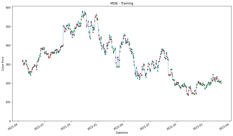
DASH
1.3655498460295028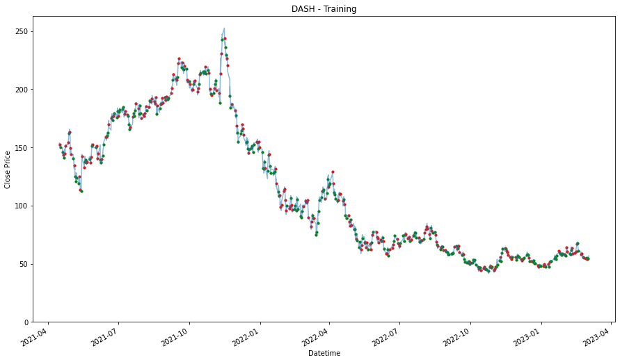
SPY
1.1370392017985178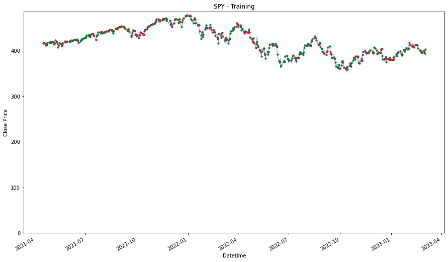
Using Testing Data
_____________________
PDD
0.962917971772168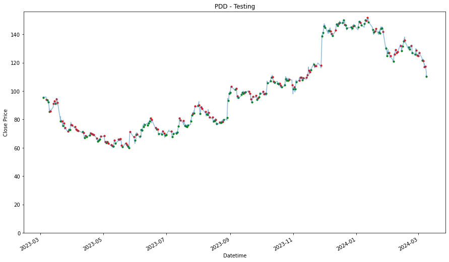
MDB
1.0033284217585219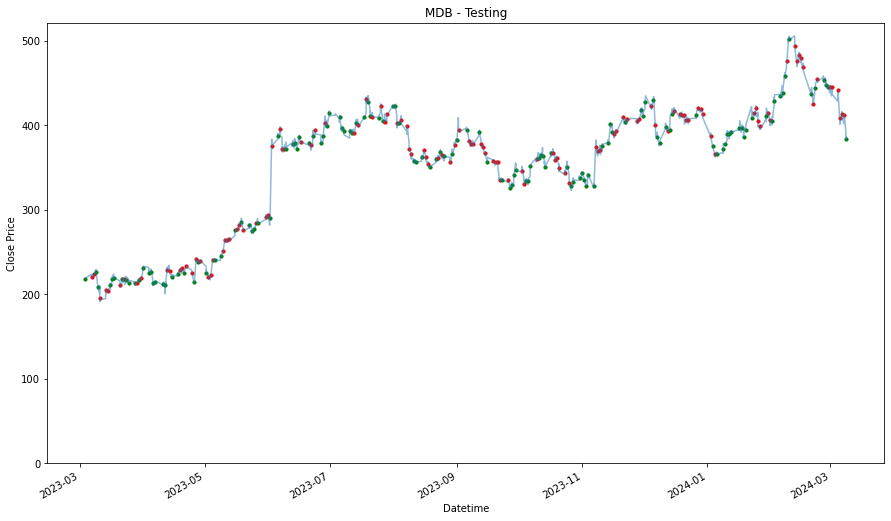
DASH
1.0128765761639726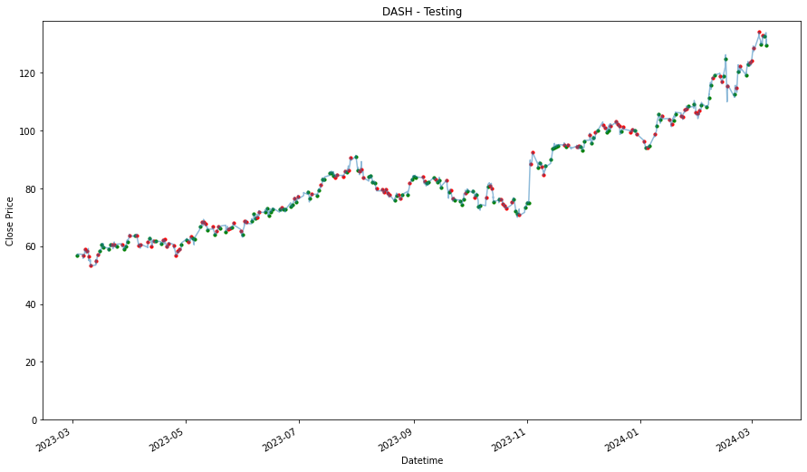
SPY
1.035842211343177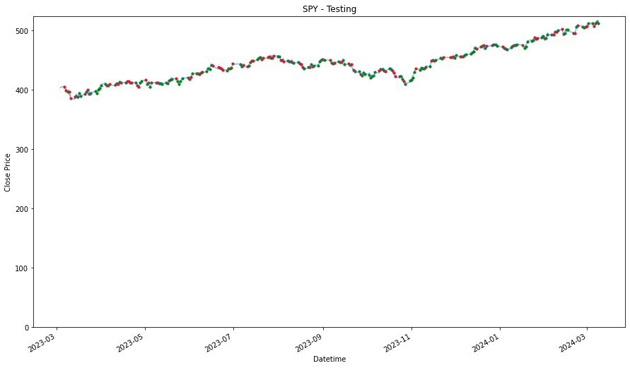
Stock Ticker                             PDD       MDB      DASH       SPY
Buy and Hold                       -0.181758  0.224945 -0.091034  0.236128
Dollar Cost Averaging (Daily)       0.489227  0.254254  0.552831  0.200805
Dollar Cost Averaging (Weekly)      0.472529  0.253272  0.556192  0.200736
Dollar Cost Averaging (Monthly)     0.503826  0.242322  0.554912  0.200701
Dollar Cost Averaging (Hourly)      0.490052  0.254119  0.552687  0.200839
General Best 3 Hours - Training     1.104347  0.900158  0.135400  0.121698
General Best 3 Hours - Testing     -0.100310  0.358737  0.478041  0.122986
General Best Hour - Training        0.389779  0.214474 -0.024389 -0.025788
General Best Hour - Testing        -0.037082  0.543056  0.468732  0.102684
Individual Best 3 Hours - Training  1.104347  0.845643  0.381333  0.162691
Individual Best 3 Hours - Testing  -0.100310  0.500780  0.646637  0.050682
Individual Best Hour - Training     0.389779  0.563103  0.365550  0.137039
Individual Best Hour - Testing     -0.037082  0.003328  0.012877  0.035842
Visualizing the Results
plt.subplots(4,1, figsize=(10,30))

for stock_no, stock in enumerate(stocks_list):

    plt.subplot(4,1,stock_no+1)

    bar_color = []
    alpha_list = []
    for i in range(5): bar_color.append('tab:blue')

    count = 0
    color_range = 1
    for i in range(5,len(performances.columns)):
        bar_color.append('C' + str(color_range))

        count += 1
        if count == 2:
            count = 0
            color_range += 1

    plt.bar(performances.columns, performances.loc[stock,:], color = bar_color)

    plt.title('Strategy Performances ' + stock)
    plt.xticks(rotation=45, ha='right')

plt.tight_layout()
plt.show()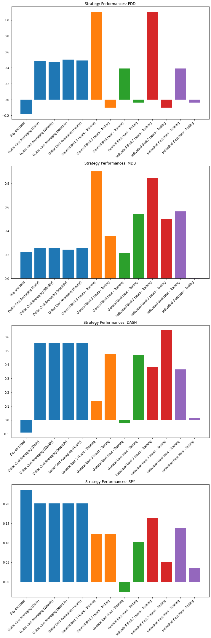
Conclusion
We collected the results and we have noted the following:
PDD
While it does seem that all the proposed strategy was not able beat dollar cost averaging, but it managed to outperform buy and hold. We may need more data to further verify this, but based on what is given, these strategies proposed, has able to beat the 'buy and hold' strategy. DCA for this dataset is so dominant because of the price movement throughout our dataset. Based on this graph, DCA will definitely be in an advantageous position as we are entering the market bit by bit, and this dataset is also the DCA strategy's best case scenario. Because DCA can perform so much better than the proposed strategies, DCA is the way to go for this stock.
MDB
All of the strategy proposed for this stock has outperformed the baseline strategies, except for the individual best hour. Ironic that the best performing hour for the individual stock in the training set, is the worst performing one in the testing set. It could be because it so happens to be on a day or hour which had a big drop in price movement. The added effort in analyzing and finding the pattern might be worth it for this stock.
DASH
We can see that DCA strategy once again is performing really well as the DASH chart is also an ideal situation for the DCA strategy. Only the individual best 3 hours outperform all the baseline strategies, with the General Best 3 Hour, and Individual best hour being close to DCA. This makes the extra effort not as worth it, when DCA can perform just as well.
SPY
Because of the steadier nature of this stock, it is harder for DCA to have an advantage over 'buy and hold'. It is worth even less for us to be putting the extra effort in spotting any patterns to take advantage of, according to the strategies that has been propose, because all of them did not perform as close as the baseline strategies proposed.
At the moment, the baseline strategies still seems attractive due to how simple and easy it is to execute, and the proposed strategy, while in some cases outperformed the baseline strategies, but not reliably. With how simple either baseline strategies are, based on what we have observed and tested, if investors would be willing to take the risks by trying to select other stocks, with a little bit of effort and some number of stock pick, just by using DCA, it is likely for them to be able to make more returns than 'buy and hold'.
Optimal Time to Hold
The above strategies, we have based our decision on a pre-determine choice that we will be only entering the market for only 1 hour, and have managed to have some interesting result. Now we will increase our data into a larger size dataset by creating a very large 'what if' table. Assuming we want to hold a trade for the maximum of 1 year, as that would be our the limit of our risk appetite, we will then create rows of percentage change in price. We will try to just use basic analytics techniques to see if we can identify any trends and pattern that we can take advantage of
The following code ran for 4 hour. The initial idea for the follow code is find out is there an optimal time to hold each of the stock. Given a limit of one year, we tried to create a dataset which consisted of the current datetime, at the current hour, match with all the subsequent datetime until the next year. And we do it for all of them.
## This was used to generate the dataset.


#for stock in stocks_list:
#    print(stock)
#
#    df = pd.concat([training_stock_data[stock], testing_stock_data[stock]])
#
#    df = df.drop(['Open', 'High', 'Low', 'Volume', 'Dividends', 'Stock Splits', '% Change in Close Price'], axis = 1)
#
#    buy_columns = 'Buy - ' + df.columns
#    sell_columns = 'Sell - ' + df.columns
#    combined_columns = buy_columns.append(sell_columns)
#
#    temp_list = []
#
#    for i in range(0,len(df)):
#
#        buy_list = list(df.iloc[i,:])
#        #print(buy_list)
#        for j in range(0, len(df)):
#
#            sell_list = list(df.iloc[j,:])
#            temp = buy_list + sell_list
#
#            time_diff = (df.iloc[j, df.columns.get_loc('Datetime')] - df.iloc[i, df.columns.get_loc('Datetime')]).days
#
#            if time_diff <= 365: temp_list.append(temp)
#
#    new_df = pd.DataFrame(temp_list, columns=combined_columns)
#    new_df.to_csv("stock_data" + "\\" + stock + " - Possible Investment Durations")
These generated data could be accessed via this link. https://www.dropbox.com/scl/fo/may2j9la0d17wtjifpdi2/h?rlkey=2luvw3aqf6t6cdc8bau7pm3vw&dl=0
new_stocks_data = {}stock_ticker = "DASH"
new_stocks_data[stock_ticker] = pd.read_csv("stock_data" + "\\" + stock_ticker + " - Possible Investment Durations")
new_stocks_data[stock_ticker] Unnamed: 0 Buy - Datetime Buy - Close Buy - Hour Buy - Day \
0 0 2021-04-15 13:30:00 151.964996 0 15
1 1 2021-04-15 13:30:00 151.964996 0 15
2 2 2021-04-15 13:30:00 151.964996 0 15
3 3 2021-04-15 13:30:00 151.964996 0 15
4 4 2021-04-15 13:30:00 151.964996 0 15
... ... ... ... ... ...
20379689 20379689 2024-03-08 19:30:00 131.300003 6 8
20379690 20379690 2024-03-08 19:30:00 131.300003 6 8
20379691 20379691 2024-03-08 19:30:00 131.300003 6 8
20379692 20379692 2024-03-08 19:30:00 131.300003 6 8
20379693 20379693 2024-03-08 19:30:00 131.300003 6 8
Buy - Day_of_Week Buy - Month Sell - Datetime Sell - Close \
0 3 4 2021-04-15 13:30:00 151.964996
1 3 4 2021-04-15 14:30:00 152.500000
2 3 4 2021-04-15 15:30:00 153.139999
3 3 4 2021-04-15 16:30:00 153.884995
4 3 4 2021-04-15 17:30:00 152.520004
... ... ... ... ...
20379689 4 3 2024-03-08 15:30:00 131.804993
20379690 4 3 2024-03-08 16:30:00 132.149994
20379691 4 3 2024-03-08 17:30:00 129.649994
20379692 4 3 2024-03-08 18:30:00 130.639999
20379693 4 3 2024-03-08 19:30:00 131.300003
Sell - Hour Sell - Day Sell - Day_of_Week Sell - Month
0 0 15 3 4
1 1 15 3 4
2 2 15 3 4
3 3 15 3 4
4 4 15 3 4
... ... ... ... ...
20379689 2 8 4 3
20379690 3 8 4 3
20379691 4 8 4 3
20379692 5 8 4 3
20379693 6 8 4 3
[20379694 rows x 13 columns]stock_ticker = "PDD"
new_stocks_data[stock_ticker] = pd.read_csv("stock_data" + "\\" + stock_ticker + " - Possible Investment Durations")
new_stocks_data[stock_ticker] Unnamed: 0 Buy - Datetime Buy - Close Buy - Hour Buy - Day \
0 0 2021-04-15 13:30:00 132.725006 0 15
1 1 2021-04-15 13:30:00 132.725006 0 15
2 2 2021-04-15 13:30:00 132.725006 0 15
3 3 2021-04-15 13:30:00 132.725006 0 15
4 4 2021-04-15 13:30:00 132.725006 0 15
... ... ... ... ... ...
20379689 20379689 2024-03-08 19:30:00 110.235001 6 8
20379690 20379690 2024-03-08 19:30:00 110.235001 6 8
20379691 20379691 2024-03-08 19:30:00 110.235001 6 8
20379692 20379692 2024-03-08 19:30:00 110.235001 6 8
20379693 20379693 2024-03-08 19:30:00 110.235001 6 8
Buy - Day_of_Week Buy - Month Sell - Datetime Sell - Close \
0 3 4 2021-04-15 13:30:00 132.725006
1 3 4 2021-04-15 14:30:00 131.229904
2 3 4 2021-04-15 15:30:00 131.320007
3 3 4 2021-04-15 16:30:00 131.639999
4 3 4 2021-04-15 17:30:00 131.929993
... ... ... ... ...
20379689 4 3 2024-03-08 15:30:00 110.879997
20379690 4 3 2024-03-08 16:30:00 110.160004
20379691 4 3 2024-03-08 17:30:00 111.099998
20379692 4 3 2024-03-08 18:30:00 110.910004
20379693 4 3 2024-03-08 19:30:00 110.235001
Sell - Hour Sell - Day Sell - Day_of_Week Sell - Month
0 0 15 3 4
1 1 15 3 4
2 2 15 3 4
3 3 15 3 4
4 4 15 3 4
... ... ... ... ...
20379689 2 8 4 3
20379690 3 8 4 3
20379691 4 8 4 3
20379692 5 8 4 3
20379693 6 8 4 3
[20379694 rows x 13 columns]stock_ticker = "SPY"
new_stocks_data[stock_ticker] = pd.read_csv("stock_data" + "\\" + stock_ticker + " - Possible Investment Durations")
new_stocks_data[stock_ticker] Unnamed: 0 Buy - Datetime Buy - Close Buy - Capital Gains \
0 0 2021-04-15 13:30:00 414.559998 0.0
1 1 2021-04-15 13:30:00 414.559998 0.0
2 2 2021-04-15 13:30:00 414.559998 0.0
3 3 2021-04-15 13:30:00 414.559998 0.0
4 4 2021-04-15 13:30:00 414.559998 0.0
... ... ... ... ...
20362483 20362483 2024-03-08 19:30:00 511.929993 0.0
20362484 20362484 2024-03-08 19:30:00 511.929993 0.0
20362485 20362485 2024-03-08 19:30:00 511.929993 0.0
20362486 20362486 2024-03-08 19:30:00 511.929993 0.0
20362487 20362487 2024-03-08 19:30:00 511.929993 0.0
Buy - Hour Buy - Day Buy - Day_of_Week Buy - Month \
0 0 15 3 4
1 0 15 3 4
2 0 15 3 4
3 0 15 3 4
4 0 15 3 4
... ... ... ... ...
20362483 6 8 4 3
20362484 6 8 4 3
20362485 6 8 4 3
20362486 6 8 4 3
20362487 6 8 4 3
Sell - Datetime Sell - Close Sell - Capital Gains \
0 2021-04-15 13:30:00 414.559998 0.0
1 2021-04-15 14:30:00 414.645691 0.0
2 2021-04-15 15:30:00 415.170013 0.0
3 2021-04-15 16:30:00 415.290009 0.0
4 2021-04-15 17:30:00 415.609985 0.0
... ... ... ...
20362483 2024-03-08 15:30:00 514.760010 0.0
20362484 2024-03-08 16:30:00 514.630005 0.0
20362485 2024-03-08 17:30:00 512.330017 0.0
20362486 2024-03-08 18:30:00 513.460022 0.0
20362487 2024-03-08 19:30:00 511.929993 0.0
Sell - Hour Sell - Day Sell - Day_of_Week Sell - Month
0 0 15 3 4
1 1 15 3 4
2 2 15 3 4
3 3 15 3 4
4 4 15 3 4
... ... ... ... ...
20362483 2 8 4 3
20362484 3 8 4 3
20362485 4 8 4 3
20362486 5 8 4 3
20362487 6 8 4 3
[20362488 rows x 15 columns]stock_ticker = "MDB"
new_stocks_data[stock_ticker] = pd.read_csv("stock_data" + "\\" + stock_ticker + " - Possible Investment Durations")
new_stocks_data[stock_ticker] Unnamed: 0 Buy - Datetime Buy - Close Buy - Hour Buy - Day \
0 0 2021-04-15 13:30:00 311.209991 0 15
1 1 2021-04-15 13:30:00 311.209991 0 15
2 2 2021-04-15 13:30:00 311.209991 0 15
3 3 2021-04-15 13:30:00 311.209991 0 15
4 4 2021-04-15 13:30:00 311.209991 0 15
... ... ... ... ... ...
20379689 20379689 2024-03-08 19:30:00 385.424988 6 8
20379690 20379690 2024-03-08 19:30:00 385.424988 6 8
20379691 20379691 2024-03-08 19:30:00 385.424988 6 8
20379692 20379692 2024-03-08 19:30:00 385.424988 6 8
20379693 20379693 2024-03-08 19:30:00 385.424988 6 8
Buy - Day_of_Week Buy - Month Sell - Datetime Sell - Close \
0 3 4 2021-04-15 13:30:00 311.209991
1 3 4 2021-04-15 14:30:00 312.670013
2 3 4 2021-04-15 15:30:00 318.079987
3 3 4 2021-04-15 16:30:00 317.605011
4 3 4 2021-04-15 17:30:00 319.959991
... ... ... ... ...
20379689 4 3 2024-03-08 15:30:00 381.812592
20379690 4 3 2024-03-08 16:30:00 386.524994
20379691 4 3 2024-03-08 17:30:00 384.000000
20379692 4 3 2024-03-08 18:30:00 384.359985
20379693 4 3 2024-03-08 19:30:00 385.424988
Sell - Hour Sell - Day Sell - Day_of_Week Sell - Month
0 0 15 3 4
1 1 15 3 4
2 2 15 3 4
3 3 15 3 4
4 4 15 3 4
... ... ... ... ...
20379689 2 8 4 3
20379690 3 8 4 3
20379691 4 8 4 3
20379692 5 8 4 3
20379693 6 8 4 3
[20379694 rows x 13 columns]After creating the large dataset, we will be removing some of the data that we will not be using neither do they make any sense. We will be pre-processing this data.
We will start to create a column that indicates the duration of holding the stock.
Then we will filter those that are equal and below 0, as that indicates purchasing the same datetime itself.
Then, we will need a column to indicate the percentage change in price.
Once we have this, we can explore to see if there are trends that we can capitalize on. Similarly, we will need to split it into training and testing once again and then put it to the test again. Because the baseline for the 'buy and hold', had a performance of +50% PDD, +25% MDB, +55% DASH, and +23% SPY. Therefore, to beat the baseline, we will need to aim to do better.
In the following code, we will prepare a list of expected return, from 3% to 75% return. Then we try to store the average duration for a entry to make that amount of profit, and also further store the most occurring buying hour and day, and also the most occurring selling hour and day. While the time is limited, we did not check and test these listed properties to see if it can beat the baseline. But the general trend noted from tht below findings is that the longer one holds the entry or investment, the more likely it is to have a higher profit.
training_period = training_stock_data['PDD']['Datetime']

return_list = [0.03, 0.05, 0.1, 0.3, 0.5, 0.65, 0.75]
optimal_strategy = pd.DataFrame(columns = ['Stock', 'Expected Return', 'Average Duration',
                                           'Buy - Hour','Buy - Day', 'Buy - Day of Week',
                                           'Sell - Hour','Sell - Day', 'Sell - Day of Week'])

for stock in stocks_list:
    print(stock)

    df = new_stocks_data[stock].copy()

    # Calculating the Duration
    # Convert the datetime from string to datetime
    df['Sell - Datetime'] = pd.to_datetime(df['Sell - Datetime'], errors='coerce', utc=True)
    df['Buy - Datetime'] = pd.to_datetime(df['Buy - Datetime'], errors='coerce', utc=True)
    df['Sell - Datetime'] = df['Sell - Datetime'].dt.tz_localize(None)
    df['Buy - Datetime'] = df['Buy - Datetime'].dt.tz_localize(None)

    # Get the duration of holding the stock
    df['Duration (Hours)'] = (df['Sell - Datetime'] - df['Buy - Datetime']) / pd.Timedelta(hours = 1)

    # Removing those that have duration of equal or less than 0
    df = df[(df['Duration (Hours)'] > 0)]

    # Calculating the percentage change in price
    df['% Change in Price'] = (df['Sell - Close'] - df['Buy - Close']) / df['Buy - Close']

    # Filter those that are in the training set
    df_train = df[(df['Sell - Datetime'] <= training_period.tail(1).item())].copy()

    # Loop expected return
    for expected_return in return_list:

        # Store the most occurring buying day/hour and selling day/hour.
        temp_df = df_train[df_train['% Change in Price'] >= expected_return].copy()
        average_duration = temp_df['Duration (Hours)'].mean()
        mode_buy_hour = temp_df['Buy - Hour'].mode()
        mode_buy_day = temp_df['Buy - Day'].mode()
        mode_buy_day_of_week = temp_df['Buy - Day_of_Week'].mode()
        mode_sell_hour = temp_df['Sell - Hour'].mode()
        mode_sell_day = temp_df['Sell - Day'].mode()
        mode_sell_day_of_week = temp_df['Sell - Day_of_Week'].mode()

        # Store them into the table
        optimal_strategy.loc[len(optimal_strategy.index)] = [stock, expected_return, average_duration,
                                          mode_buy_hour, mode_buy_day, mode_buy_day_of_week,
                                          mode_sell_hour, mode_sell_day, mode_sell_day_of_week]

optimal_strategy
PDD
MDB
DASH
SPY Stock Expected Return Average Duration \
0 PDD 0.03 3757.000516
1 PDD 0.05 3826.572919
2 PDD 0.10 3978.323944
3 PDD 0.30 4417.653129
4 PDD 0.50 4904.750649
5 PDD 0.65 5254.390759
6 PDD 0.75 5557.023504
7 MDB 0.03 3033.286414
8 MDB 0.05 3093.602709
9 MDB 0.10 3235.473729
10 MDB 0.30 3649.104038
11 MDB 0.50 4229.355688
12 MDB 0.65 4407.726249
13 MDB 0.75 4388.833449
14 DASH 0.03 2010.721397
15 DASH 0.05 2063.361792
16 DASH 0.10 2197.194164
17 DASH 0.30 2954.526927
18 DASH 0.50 3440.912500
19 DASH 0.65 3779.710158
20 DASH 0.75 3865.734914
21 SPY 0.03 3321.667364
22 SPY 0.05 3589.225845
23 SPY 0.10 4283.918912
24 SPY 0.30 NaN
25 SPY 0.50 NaN
26 SPY 0.65 NaN
27 SPY 0.75 NaN
Buy - Hour \
0 0 3
Name: Buy - Hour, dtype: int64
1 0 3
Name: Buy - Hour, dtype: int64
2 0 3
Name: Buy - Hour, dtype: int64
3 0 3
Name: Buy - Hour, dtype: int64
4 0 4
Name: Buy - Hour, dtype: int64
5 0 4
Name: Buy - Hour, dtype: int64
6 0 6
Name: Buy - Hour, dtype: int64
7 0 3
Name: Buy - Hour, dtype: int64
8 0 3
Name: Buy - Hour, dtype: int64
9 0 3
Name: Buy - Hour, dtype: int64
10 0 1
Name: Buy - Hour, dtype: int64
11 0 4
Name: Buy - Hour, dtype: int64
12 0 4
Name: Buy - Hour, dtype: int64
13 0 1
Name: Buy - Hour, dtype: int64
14 0 3
Name: Buy - Hour, dtype: int64
15 0 5
Name: Buy - Hour, dtype: int64
16 0 3
Name: Buy - Hour, dtype: int64
17 0 5
Name: Buy - Hour, dtype: int64
18 0 4
Name: Buy - Hour, dtype: int64
19 0 4
Name: Buy - Hour, dtype: int64
20 0 4
Name: Buy - Hour, dtype: int64
21 0 3
Name: Buy - Hour, dtype: int64
22 0 3
Name: Buy - Hour, dtype: int64
23 0 0
Name: Buy - Hour, dtype: int64
24 Series([], Name: Buy - Hour, dtype: int64)
25 Series([], Name: Buy - Hour, dtype: int64)
26 Series([], Name: Buy - Hour, dtype: int64)
27 Series([], Name: Buy - Hour, dtype: int64)
Buy - Day \
0 0 28
Name: Buy - Day, dtype: int64
1 0 28
Name: Buy - Day, dtype: int64
2 0 28
Name: Buy - Day, dtype: int64
3 0 11
Name: Buy - Day, dtype: int64
4 0 11
Name: Buy - Day, dtype: int64
5 0 11
Name: Buy - Day, dtype: int64
6 0 11
Name: Buy - Day, dtype: int64
7 0 28
Name: Buy - Day, dtype: int64
8 0 28
Name: Buy - Day, dtype: int64
9 0 28
Name: Buy - Day, dtype: int64
10 0 19
Name: Buy - Day, dtype: int64
11 0 19
Name: Buy - Day, dtype: int64
12 0 3
Name: Buy - Day, dtype: int64
13 0 3
Name: Buy - Day, dtype: int64
14 0 7
Name: Buy - Day, dtype: int64
15 0 3
Name: Buy - Day, dtype: int64
16 0 3
Name: Buy - Day, dtype: int64
17 0 7
Name: Buy - Day, dtype: int64
18 0 13
Name: Buy - Day, dtype: int64
19 0 13
Name: Buy - Day, dtype: int64
20 0 13
Name: Buy - Day, dtype: int64
21 0 21
Name: Buy - Day, dtype: int64
22 0 21
Name: Buy - Day, dtype: int64
23 0 19
Name: Buy - Day, dtype: int64
24 Series([], Name: Buy - Day, dtype: int64)
25 Series([], Name: Buy - Day, dtype: int64)
26 Series([], Name: Buy - Day, dtype: int64)
27 Series([], Name: Buy - Day, dtype: int64)
Buy - Day of Week \
0 0 3
Name: Buy - Day_of_Week, dtype: int64
1 0 3
Name: Buy - Day_of_Week, dtype: int64
2 0 3
Name: Buy - Day_of_Week, dtype: int64
3 0 3
Name: Buy - Day_of_Week, dtype: int64
4 0 3
Name: Buy - Day_of_Week, dtype: int64
5 0 3
Name: Buy - Day_of_Week, dtype: int64
6 0 1
Name: Buy - Day_of_Week, dtype: int64
7 0 3
Name: Buy - Day_of_Week, dtype: int64
8 0 3
Name: Buy - Day_of_Week, dtype: int64
9 0 3
Name: Buy - Day_of_Week, dtype: int64
10 0 1
Name: Buy - Day_of_Week, dtype: int64
11 0 3
Name: Buy - Day_of_Week, dtype: int64
12 0 3
Name: Buy - Day_of_Week, dtype: int64
13 0 3
Name: Buy - Day_of_Week, dtype: int64
14 0 3
Name: Buy - Day_of_Week, dtype: int64
15 0 3
Name: Buy - Day_of_Week, dtype: int64
16 0 3
Name: Buy - Day_of_Week, dtype: int64
17 0 3
Name: Buy - Day_of_Week, dtype: int64
18 0 3
Name: Buy - Day_of_Week, dtype: int64
19 0 3
Name: Buy - Day_of_Week, dtype: int64
20 0 3
Name: Buy - Day_of_Week, dtype: int64
21 0 3
Name: Buy - Day_of_Week, dtype: int64
22 0 3
Name: Buy - Day_of_Week, dtype: int64
23 0 3
Name: Buy - Day_of_Week, dtype: int64
24 Series([], Name: Buy - Day_of_Week, dtype: int64)
25 Series([], Name: Buy - Day_of_Week, dtype: int64)
26 Series([], Name: Buy - Day_of_Week, dtype: int64)
27 Series([], Name: Buy - Day_of_Week, dtype: int64)
Sell - Hour \
0 0 2
Name: Sell - Hour, dtype: int64
1 0 2
Name: Sell - Hour, dtype: int64
2 0 2
Name: Sell - Hour, dtype: int64
3 0 1
Name: Sell - Hour, dtype: int64
4 0 1
Name: Sell - Hour, dtype: int64
5 0 1
Name: Sell - Hour, dtype: int64
6 0 1
Name: Sell - Hour, dtype: int64
7 0 1
Name: Sell - Hour, dtype: int64
8 0 1
Name: Sell - Hour, dtype: int64
9 0 1
Name: Sell - Hour, dtype: int64
10 0 1
Name: Sell - Hour, dtype: int64
11 0 1
Name: Sell - Hour, dtype: int64
12 0 1
Name: Sell - Hour, dtype: int64
13 0 1
Name: Sell - Hour, dtype: int64
14 0 1
Name: Sell - Hour, dtype: int64
15 0 1
Name: Sell - Hour, dtype: int64
16 0 1
Name: Sell - Hour, dtype: int64
17 0 2
Name: Sell - Hour, dtype: int64
18 0 1
1 2
Name: Sell - Hour, dtype: int64
19 0 1
Name: Sell - Hour, dtype: int64
20 0 2
Name: Sell - Hour, dtype: int64
21 0 1
Name: Sell - Hour, dtype: int64
22 0 2
Name: Sell - Hour, dtype: int64
23 0 6
Name: Sell - Hour, dtype: int64
24 Series([], Name: Sell - Hour, dtype: int64)
25 Series([], Name: Sell - Hour, dtype: int64)
26 Series([], Name: Sell - Hour, dtype: int64)
27 Series([], Name: Sell - Hour, dtype: int64)
Sell - Day \
0 0 1
Name: Sell - Day, dtype: int64
1 0 1
Name: Sell - Day, dtype: int64
2 0 1
Name: Sell - Day, dtype: int64
3 0 6
Name: Sell - Day, dtype: int64
4 0 6
Name: Sell - Day, dtype: int64
5 0 9
Name: Sell - Day, dtype: int64
6 0 13
Name: Sell - Day, dtype: int64
7 0 22
Name: Sell - Day, dtype: int64
8 0 22
Name: Sell - Day, dtype: int64
9 0 8
Name: Sell - Day, dtype: int64
10 0 22
Name: Sell - Day, dtype: int64
11 0 15
Name: Sell - Day, dtype: int64
12 0 22
Name: Sell - Day, dtype: int64
13 0 22
Name: Sell - Day, dtype: int64
14 0 15
Name: Sell - Day, dtype: int64
15 0 15
Name: Sell - Day, dtype: int64
16 0 15
Name: Sell - Day, dtype: int64
17 0 15
Name: Sell - Day, dtype: int64
18 0 15
Name: Sell - Day, dtype: int64
19 0 15
Name: Sell - Day, dtype: int64
20 0 15
Name: Sell - Day, dtype: int64
21 0 1
Name: Sell - Day, dtype: int64
22 0 10
Name: Sell - Day, dtype: int64
23 0 10
Name: Sell - Day, dtype: int64
24 Series([], Name: Sell - Day, dtype: int64)
25 Series([], Name: Sell - Day, dtype: int64)
26 Series([], Name: Sell - Day, dtype: int64)
27 Series([], Name: Sell - Day, dtype: int64)
Sell - Day of Week
0 0 1
Name: Sell - Day_of_Week, dtype: int64
1 0 1
Name: Sell - Day_of_Week, dtype: int64
2 0 1
Name: Sell - Day_of_Week, dtype: int64
3 0 1
Name: Sell - Day_of_Week, dtype: int64
4 0 3
Name: Sell - Day_of_Week, dtype: int64
5 0 3
Name: Sell - Day_of_Week, dtype: int64
6 0 3
Name: Sell - Day_of_Week, dtype: int64
7 0 2
Name: Sell - Day_of_Week, dtype: int64
8 0 2
Name: Sell - Day_of_Week, dtype: int64
9 0 2
Name: Sell - Day_of_Week, dtype: int64
10 0 2
Name: Sell - Day_of_Week, dtype: int64
11 0 1
Name: Sell - Day_of_Week, dtype: int64
12 0 1
Name: Sell - Day_of_Week, dtype: int64
13 0 3
Name: Sell - Day_of_Week, dtype: int64
14 0 2
Name: Sell - Day_of_Week, dtype: int64
15 0 2
Name: Sell - Day_of_Week, dtype: int64
16 0 3
Name: Sell - Day_of_Week, dtype: int64
17 0 3
Name: Sell - Day_of_Week, dtype: int64
18 0 4
Name: Sell - Day_of_Week, dtype: int64
19 0 4
Name: Sell - Day_of_Week, dtype: int64
20 0 4
Name: Sell - Day_of_Week, dtype: int64
21 0 2
Name: Sell - Day_of_Week, dtype: int64
22 0 2
Name: Sell - Day_of_Week, dtype: int64
23 0 2
Name: Sell - Day_of_Week, dtype: int64
24 Series([], Name: Sell - Day_of_Week, dtype: in...
25 Series([], Name: Sell - Day_of_Week, dtype: in...
26 Series([], Name: Sell - Day_of_Week, dtype: in...
27 Series([], Name: Sell - Day_of_Week, dtype: in...By making some small adjustment to the return expectation, in the code below, it consists of 3% to 5%, we can now have a different sets of outcome we can test.
training_period = training_stock_data['PDD']['Datetime']

optimal_strategy = pd.DataFrame(columns = ['Stock', 'Expected Return', 'Average Duration',
                                           'Buy - Hour','Buy - Day', 'Buy - Day of Week',
                                           'Sell - Hour','Sell - Day', 'Sell - Day of Week'])

for stock in stocks_list:
    print(stock)

    df = new_stocks_data[stock].copy()

    # Calculating the Duration
    # Convert the datetime from string to datetime
    df['Sell - Datetime'] = pd.to_datetime(df['Sell - Datetime'], errors='coerce', utc=True)
    df['Buy - Datetime'] = pd.to_datetime(df['Buy - Datetime'], errors='coerce', utc=True)
    df['Sell - Datetime'] = df['Sell - Datetime'].dt.tz_localize(None)
    df['Buy - Datetime'] = df['Buy - Datetime'].dt.tz_localize(None)

    # Get the duration of holding the stock
    df['Duration (Hours)'] = (df['Sell - Datetime'] - df['Buy - Datetime']) / pd.Timedelta(hours = 1)

    # Removing those that have duration of equal or less than 0
    df = df[(df['Duration (Hours)'] > 0)]

    # Calculating the percentage change in price
    df['% Change in Price'] = (df['Sell - Close'] - df['Buy - Close']) / df['Buy - Close']

    # Filter those that are in the training set
    df_train = df[(df['Sell - Datetime'] <= training_period.tail(1).item())].copy()

    # Store the most occurring buying day/hour and selling day/hour.
    temp_df = df_train[(df_train['% Change in Price'] >= 0.03) & (df_train['% Change in Price'] <= 0.05)].copy()
    average_duration = temp_df['Duration (Hours)'].mean()
    mode_buy_hour = temp_df['Buy - Hour'].mode()
    mode_buy_day = temp_df['Buy - Day'].mode()
    mode_buy_day_of_week = temp_df['Buy - Day_of_Week'].mode()
    mode_sell_hour = temp_df['Sell - Hour'].mode()
    mode_sell_day = temp_df['Sell - Day'].mode()
    mode_sell_day_of_week = temp_df['Sell - Day_of_Week'].mode()

    # Store them into the table
    optimal_strategy.loc[len(optimal_strategy.index)] = [stock, "3% - 5%", average_duration,
                                        mode_buy_hour, mode_buy_day, mode_buy_day_of_week,
                                        mode_sell_hour, mode_sell_day, mode_sell_day_of_week]

optimal_strategyPDDMDB
DASH
SPY Stock Expected Return Average Duration \
0 PDD 3% - 5% 2252.110473
1 MDB 3% - 5% 2077.244112
2 DASH 3% - 5% 1454.757564
3 SPY 3% - 5% 2779.621244
Buy - Hour \
0 0 2
Name: Buy - Hour, dtype: int64
1 0 5
Name: Buy - Hour, dtype: int64
2 0 4
Name: Buy - Hour, dtype: int64
3 0 4
Name: Buy - Hour, dtype: int64
Buy - Day \
0 0 10
1 14
Name: Buy - Day, dtype: int64
1 0 21
Name: Buy - Day, dtype: int64
2 0 28
Name: Buy - Day, dtype: int64
3 0 21
Name: Buy - Day, dtype: int64
Buy - Day of Week \
0 0 2
Name: Buy - Day_of_Week, dtype: int64
1 0 1
Name: Buy - Day_of_Week, dtype: int64
2 0 2
Name: Buy - Day_of_Week, dtype: int64
3 0 2
Name: Buy - Day_of_Week, dtype: int64
Sell - Hour \
0 0 1
Name: Sell - Hour, dtype: int64
1 0 5
Name: Sell - Hour, dtype: int64
2 0 1
Name: Sell - Hour, dtype: int64
3 0 6
Name: Sell - Hour, dtype: int64
Sell - Day \
0 0 7
Name: Sell - Day, dtype: int64
1 0 28
Name: Sell - Day, dtype: int64
2 0 9
Name: Sell - Day, dtype: int64
3 0 1
Name: Sell - Day, dtype: int64
Sell - Day of Week
0 0 1
Name: Sell - Day_of_Week, dtype: int64
1 0 4
Name: Sell - Day_of_Week, dtype: int64
2 0 1
Name: Sell - Day_of_Week, dtype: int64
3 0 2
Name: Sell - Day_of_Week, dtype: int64But because we can see that the average duration is long, we can further tweak and add another conditions, such that we might want to only hold at the maximum of 2 weeks, which is 10 days for 8 hours, so 80 hours. Having these conditons to filter, we can then further explore with different methods to see if we can find recurring patterns or an edge in the market, but according to the investors' appetite.
training_period = training_stock_data['PDD']['Datetime']

optimal_strategy = pd.DataFrame(columns = ['Stock', 'Expected Return', 'Average Duration',
                                           'Buy - Hour','Buy - Day', 'Buy - Day of Week',
                                           'Sell - Hour','Sell - Day', 'Sell - Day of Week'])

for stock in stocks_list:
    print(stock)

    df = new_stocks_data[stock].copy()

    # Calculating the Duration
    # Convert the datetime from string to datetime
    df['Sell - Datetime'] = pd.to_datetime(df['Sell - Datetime'], errors='coerce', utc=True)
    df['Buy - Datetime'] = pd.to_datetime(df['Buy - Datetime'], errors='coerce', utc=True)
    df['Sell - Datetime'] = df['Sell - Datetime'].dt.tz_localize(None)
    df['Buy - Datetime'] = df['Buy - Datetime'].dt.tz_localize(None)

    # Get the duration of holding the stock
    df['Duration (Hours)'] = (df['Sell - Datetime'] - df['Buy - Datetime']) / pd.Timedelta(hours = 1)

    # Removing those that have duration of equal or less than 0
    df = df[(df['Duration (Hours)'] > 0)]

    # Calculating the percentage change in price
    df['% Change in Price'] = (df['Sell - Close'] - df['Buy - Close']) / df['Buy - Close']

    # Filter those that are in the training set
    df_train = df[(df['Sell - Datetime'] <= training_period.tail(1).item())].copy()

    # Store the most occurring buying day/hour and selling day/hour.
    temp_df = df_train[(df_train['% Change in Price'] >= 0.03) & (df_train['% Change in Price'] <= 0.05)].copy()
    temp_df = df_train[(df_train['Duration (Hours)'] <= 80)]
    average_duration = temp_df['Duration (Hours)'].mean()
    mode_buy_hour = temp_df['Buy - Hour'].mode()
    mode_buy_day = temp_df['Buy - Day'].mode()
    mode_buy_day_of_week = temp_df['Buy - Day_of_Week'].mode()
    mode_sell_hour = temp_df['Sell - Hour'].mode()
    mode_sell_day = temp_df['Sell - Day'].mode()
    mode_sell_day_of_week = temp_df['Sell - Day_of_Week'].mode()

    # Store them into the table
    optimal_strategy.loc[len(optimal_strategy.index)] = [stock, "3% - 5%", average_duration,
                                        mode_buy_hour, mode_buy_day, mode_buy_day_of_week,
                                        mode_sell_hour, mode_sell_day, mode_sell_day_of_week]

optimal_strategyPDDMDB
DASH
SPY Stock Expected Return Average Duration \
0 PDD 3% - 5% 37.257470
1 MDB 3% - 5% 37.257470
2 DASH 3% - 5% 37.257470
3 SPY 3% - 5% 37.247091
Buy - Hour \
0 0 1
Name: Buy - Hour, dtype: int64
1 0 1
Name: Buy - Hour, dtype: int64
2 0 1
Name: Buy - Hour, dtype: int64
3 0 1
Name: Buy - Hour, dtype: int64
Buy - Day \
0 0 28
Name: Buy - Day, dtype: int64
1 0 28
Name: Buy - Day, dtype: int64
2 0 28
Name: Buy - Day, dtype: int64
3 0 28
Name: Buy - Day, dtype: int64
Buy - Day of Week \
0 0 1
Name: Buy - Day_of_Week, dtype: int64
1 0 1
Name: Buy - Day_of_Week, dtype: int64
2 0 1
Name: Buy - Day_of_Week, dtype: int64
3 0 1
Name: Buy - Day_of_Week, dtype: int64
Sell - Hour \
0 0 6
Name: Sell - Hour, dtype: int64
1 0 6
Name: Sell - Hour, dtype: int64
2 0 6
Name: Sell - Hour, dtype: int64
3 0 6
Name: Sell - Hour, dtype: int64
Sell - Day \
0 0 23
Name: Sell - Day, dtype: int64
1 0 23
Name: Sell - Day, dtype: int64
2 0 23
Name: Sell - Day, dtype: int64
3 0 23
Name: Sell - Day, dtype: int64
Sell - Day of Week
0 0 4
Name: Sell - Day_of_Week, dtype: int64
1 0 4
Name: Sell - Day_of_Week, dtype: int64
2 0 4
Name: Sell - Day_of_Week, dtype: int64
3 0 4
Name: Sell - Day_of_Week, dtype: int64In conclusion, while we might not have tested the findings we have here due to time constraint, it is definitely an area that could be further looked into, and might need to adopt some form of pattern recognizer to automatically seek out formulas or trends might not be obvious to us, such as using Genetic Algorithm, Path Finding/Search Algorithms or Clustering Algorithms.
This new set of data that was created seems like a good way to also further preprocess into many other forms of data. For example, we could remove the datetime and leave the rest of the data. Then make the duration a target variable for a machine learning model to train and it might be able to guess how long we will need to hold the stock for a certain percentage of return, given the current set of datetime information. Similar to what is shown in the coursework 1 section, where we tried to look for recurring patterns but looking into past a fixed number of periods, what kind of property of the price movement can lead that might lead to the returns that an investor can expect.