Predicting Financial Well-Being - A Socioeconomic Analysis using Bayesian Networks

Introduction

The primary goal of this Decision Support System is to improve decision making by identifying patterns in historical data and predicting key attributes. This project focuses on developing a system that evaluates the financial literacy and behaviour of an individual. These assessments are based on socioeconomic factors such as gender and age along with educational attainment. The resulting scores are then used to predict the overall financial well-being of the individual.

The data for this system comes from a questionnaire conducted in Romania during 2022 by Mihai Nitoi. This study collected socioeconomic information to explore how literacy and behaviour relate to financial well-being. This analysis uses the same dataset as a previous study which can be found in this project post.

This project follows a structured approach based on the specific requirements of the coursework. The details are organized into several tasks that lead toward a final implementation.

Task 1 - Conceptual Design of a Decision Support System

Purpose

This system offers valuable insights that support better financial decisions. It determines levels of literacy and behaviour to provide a clear picture of financial health. This tool can serve as a helpful module for larger systems used by financial institutions. It can assist in evaluating risk ratings or providing personalized investment recommendations to clients.

Specifications

• Task: The project develops a system using a dataset from a Romanian questionnaire to explore how socioeconomic factors influence financial outcomes. One main objective is to establish the levels of literacy and well-being based on the background of an individual. It can also work in reverse by predicting socioeconomic traits from known financial scores.

• Objective:The system is designed to be a supporting component for extensive financial models. For example a bank could use it to assess credit risk during loan applications or to find suitable investment products for different customers. There are some limitations to consider when using the system. The model relies on data from a specific group in Romania so its findings apply most accurately to that demographic. A more diverse dataset would be necessary to extend these results to other regions. The sample size includes approximately 1,400 participants which is useful for study but might require more data for a large scale production environment.

Data and Knowledge Requirements

A basic understanding of finance is helpful when using the system. It can be difficult to interpret the results without some prior knowledge of these concepts. The sociodemographic data requires straightforward processing but calculating the scores for literacy and well-being involves more detail.

The literacy score is found by combining answers to specific questions. Financial behaviour is measured by ranking various habits and aggregating them into a single result. The well-being score follows a established method from the research of Mihai Nitoi and the Consumer Financial Protection Bureau.

The current model uses factors such as age and educational attainment. The dataset also contains other details like employment status and household size which could be added in the future. These additions would make the analysis even more comprehensive. Extending the model to include different regions is also possible by adding new data sources and regional identifiers. The metrics used in this project are based on trusted global standards which makes the system reliable and easy to adapt.

Users and Potential Stakeholders

Researchers and financial institutions are the primary users of this system. Regulatory bodies can also benefit from these insights. These groups can use the tool to estimate the probability of various financial outcomes based on demographic data.

Researchers can use this system as a standard for comparisons in their studies. For financial institutions the outputs can guide important choices about credit ratings and loan approvals. It can also help with creating better marketing strategies and optimizing financial products for customers. Organizations that have large amounts of data can further improve the utility of this system by integrating their own records.

Integrating the System

This system can work on its own to provide useful probabilities and insights. It is even more effective when used alongside other models to support complex decision making. In a scenario like investment planning a bank might combine several different models. They could use one system to check transaction history and another to evaluate risk profiles. This decision support tool would then provide additional details about literacy and well-being to help advisors create appropriate plans for their clients.

Task 2 Development of a simple Bayesian Network

Textual Description

The following graph illustrates the Bayesian network designed for this project.

The model identifies sociodemographic factors as the primary drivers of financial literacy and behaviour. As an individual grows older their literacy and behaviour scores are likely to improve because of the natural progression of life and increasing responsibilities. Older individuals often gain more experience which helps them become more financially responsible and knowledgeable.

Educational attainment follows a similar logic because higher levels of education typically correlate with better financial understanding. Gender is also considered as historical data shows that women sometimes had fewer opportunities for higher education. This factor might result in lower scores for older women in certain demographics. The model also establishes that literacy and behaviour are direct causes of financial well-being. Individuals with higher scores in these areas are better equipped to make sound financial choices and maintain healthy habits. The following section explores the probabilities associated with each component of the network.

Nodes Exploration

Gender

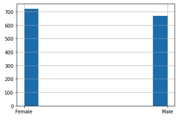
The dataset includes 722 females and 669 males. This distribution results in a probability of 0.52 for females and 0.48 for males.

Age

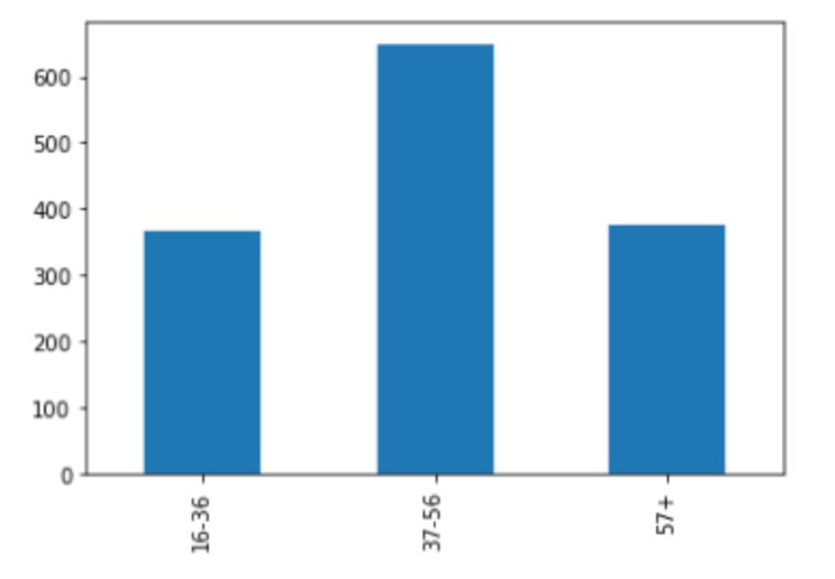
The age attribute is simplified by dividing participants into three distinct groups. These groups include individuals from 16 to 36 years old and 37 to 56 years old as well as those 57 and older. There are 366 participants in the first group and 650 in the second while the remaining 375 are in the third group.

Education Attainment

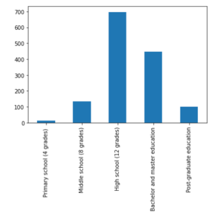
The majority of participants have completed high school or a bachelor degree while fewer individuals are at the opposite ends of the educational spectrum. We decided to group these levels for a clearer analysis.

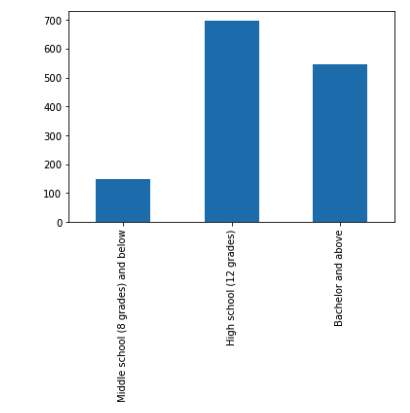
After combining the categories there are 147 participants with middle school education or lower and 697 who completed high school. Another 547 individuals have earned a bachelor degree or higher. This results in a distribution of 0.11 and 0.50 and 0.39 respectively.

Financial Behaviour

The questionnaire included several questions about financial habits but we focused on two specific areas for this model. These areas involve the practice of keep financial records and the types of instruments used for investments. The responses were used to calculate a final score for each individual.

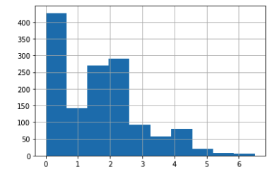
The results are divided into three groups based on their scores. These categories include scores from 0 to 2 and 2 to 4 as well as those above 4.

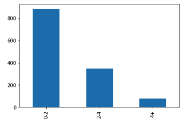
The distribution for these categories is 0.6937 for the lowest group and 0.2495 for the middle group while the highest group has a probability of 0.0568.

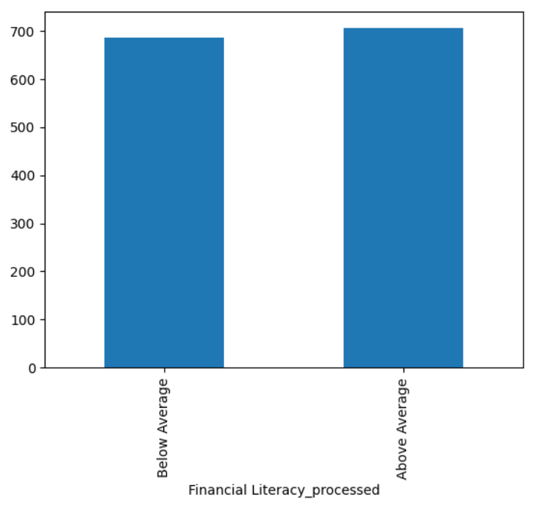
Financial Literacy

Financial literacy is measured through eight different questions. We followed a scoring method provided by Mihai Nitoi and aggregated the results by summing them together.

The project eventually categorized literacy into levels of Below Average and Above Average. This simplification was necessary to ensure the model could produce clear outcomes during the later stages of inference.

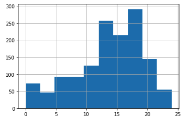
Financial Well Being

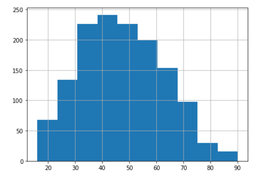
Finally the well being score is derived from ten questions about financial stability. These scores are matched against a reference table that accounts for different response patterns. The following histogram shows the initial distribution of these scores.

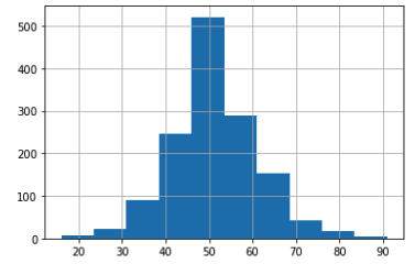
Participants was initially divided into five categories ranging from very low to very high.

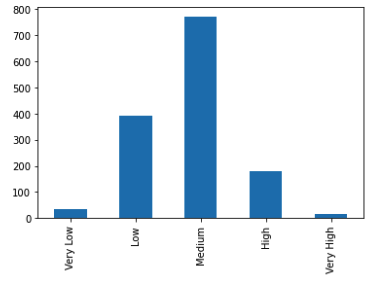
During the final development of the project we consolidated these into three categories for better model performance.

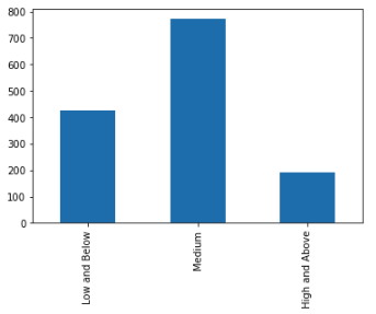
The final arrangement uses three groups with probabilities of 0.307 for Low and Below and 0.554 for Medium as well as 0.139 for High and Above.

Task 3 Implementation in Python

Model Definition

Now that the parameters are prepared we can begin building the Bayesian network in Python. We start by defining the structure of the network according to the design outlined in the previous section.

model = BayesianNetwork(
    [
        ('Gender', 'Financial Literacy'),
        ('Gender', 'Financial Behaviour'),
        ('Age', 'Financial Literacy'),
        ('Age', 'Financial Behaviour'),
        ('Education', 'Financial Literacy'),
        ('Education', 'Financial Behaviour'),
        ('Financial Literacy', 'Financial Well Being'),
        ('Financial Behaviour', 'Financial Well Being')
    ]
)

We then use the probabilities established earlier to define the individual nodes of the model.

Defining Conditional Probability Distributions

Gender Probability

gender_cpd = TabularCPD(
    variable='Gender',
    variable_card=2,
    values = [[0.519051],[0.480949]],
    state_names={
        'Gender':[
            'Female',
            'Male'
        ]
    }
)
model.add_cpds(gender_cpd)

print(model.get_cpds('Gender'))

+----------------+----------+
| Gender(Female) | 0.519051 |
+----------------+----------+
| Gender(Male)   | 0.480949 |
+----------------+----------+

Age Probability

age_cpd = TabularCPD(
    variable='Age',
    variable_card=3,
    values=[
        [0.26312],[0.46729],[0.26959]
    ],
    state_names={
        'Age':[
            '16-36', '37-56', '76+'
        ]
    }
)
model.add_cpds(age_cpd)

print(model.get_cpds('Age'))

+------------+---------+
| Age(16-36) | 0.26312 |
+------------+---------+
| Age(37-56) | 0.46729 |
+------------+---------+
| Age(76+)   | 0.26959 |
+------------+---------+

Education Probability

income_cpd = TabularCPD(
    variable='Education',
    variable_card=3,
    values=[
        [0.3932],[0.5011],[0.1057],
    ],
    state_names={
        'Education':[
            'Middle school (8 grades) and below',
            'High school (12 grades)',
            'Bachelor and above',
        ]
    }
)
model.add_cpds(income_cpd)

print(model.get_cpds('Education'))

+-----------------------------------------------+--------+
| Education(Middle school (8 grades) and below) | 0.3932 |
+-----------------------------------------------+--------+
| Education(High school (12 grades))            | 0.5011 |
+-----------------------------------------------+--------+
| Education(Bachelor and above)                 | 0.1057 |
+-----------------------------------------------+--------+

Financial Literacy Probability

The probabilities are calculated based on the influence of sociodemographic factors.

FL_socio_probability = pd.crosstab(
    df['Financial Literacy_processed'],
    [df['SD2'],df['SD3_processed'],df['SD4_processed']],
    normalize='columns',dropna=False,margins=True
)

Financial Literacy_processed	('Female', '16-36', 'Bachelor and above')	('Female', '16-36', 'High school (12 grades)')	('Female', '16-36', 'Middle school (8 grades) and below')	('Female', '37-56', 'Bachelor and above')	('Female', '37-56', 'High school (12 grades)')	('Female', '37-56', 'Middle school (8 grades) and below')	('Female', '57+', 'Bachelor and above')	('Female', '57+', 'High school (12 grades)')	('Female', '57+', 'Middle school (8 grades) and below')	('Male', '16-36', 'Bachelor and above')	('Male', '16-36', 'High school (12 grades)')	('Male', '16-36', 'Middle school (8 grades) and below')	('Male', '37-56', 'Bachelor and above')	('Male', '37-56', 'High school (12 grades)')	('Male', '37-56', 'Middle school (8 grades) and below')	('Male', '57+', 'Bachelor and above')	('Male', '57+', 'High school (12 grades)')	('Male', '57+', 'Middle school (8 grades) and below')	('All', '', '')
Below Average	0.344828	0.430556	0.625	0.322581	0.48538	0.923077	0.347826	0.764706	0.94	0.243243	0.403509	0.8	0.363636	0.494624	0.846154	0.333333	0.634921	0.975	0.49317
Above Average	0.655172	0.569444	0.375	0.677419	0.51462	0.0769231	0.652174	0.235294	0.06	0.756757	0.596491	0.2	0.636364	0.505376	0.153846	0.666667	0.365079	0.025	0.50683

We then incorporate these calculated values into the network model.

FL_socio_cpd = TabularCPD(
    variable='Financial Literacy',
    variable_card=2,
    evidence=['Gender', 'Age','Education'],
    evidence_card=distinct_value_count_for_socio_col,
    values = [
        [x for x in FL_socio_probability.loc['Below Average'][:-1]],
        [x for x in FL_socio_probability.loc['Above Average'][:-1]]
    ],

    state_names={
        'Financial Literacy':[x for x in FL_socio_probability.index],

        'Age':[
            '16-36', '37-56', '76+'
        ],

        'Gender':[
            'Female',
            'Male'
        ],

        'Education':[
            'Middle school (8 grades) and below',
            'High school (12 grades)',
            'Bachelor and above',
        ]
    }
)
model.add_cpds(FL_socio_cpd)

print(model.get_cpds('Financial Literacy'))

+-----------------------------------+-----+-------------------------------+
| Gender                            | ... | Gender(Male)                  |
+-----------------------------------+-----+-------------------------------+
| Age                               | ... | Age(76+)                      |
+-----------------------------------+-----+-------------------------------+
| Education                         | ... | Education(Bachelor and above) |
+-----------------------------------+-----+-------------------------------+
| Financial Literacy(Below Average) | ... | 0.975                         |
+-----------------------------------+-----+-------------------------------+
| Financial Literacy(Above Average) | ... | 0.025                         |
+-----------------------------------+-----+-------------------------------+

Financial Behaviour Probability

Similarly for FB, will get the list of probabilities. Then include it into the network.

FB_socio_probability = pd.crosstab(
    df['Financial Behaviour'],
    [df['SD2'],df['SD3_processed'],df['SD4_processed']],
    normalize='columns',dropna=False,margins=True
)

Financial Behaviour	('Female', '16-36', 'Bachelor and above')	('Female', '16-36', 'High school (12 grades)')	('Female', '16-36', 'Middle school (8 grades) and below')	('Female', '37-56', 'Bachelor and above')	('Female', '37-56', 'High school (12 grades)')	('Female', '37-56', 'Middle school (8 grades) and below')	('Female', '57+', 'Bachelor and above')	('Female', '57+', 'High school (12 grades)')	('Female', '57+', 'Middle school (8 grades) and below')	('Male', '16-36', 'Bachelor and above')	('Male', '16-36', 'High school (12 grades)')	('Male', '16-36', 'Middle school (8 grades) and below')	('Male', '37-56', 'Bachelor and above')	('Male', '37-56', 'High school (12 grades)')	('Male', '37-56', 'Middle school (8 grades) and below')	('Male', '57+', 'Bachelor and above')	('Male', '57+', 'High school (12 grades)')	('Male', '57+', 'Middle school (8 grades) and below')	('All', '', '')
0-2	0.537931	0.736111	1	0.445161	0.754386	0.846154	0.608696	0.776471	0.8	0.486486	0.842105	1	0.585859	0.833333	0.961538	0.490196	0.81746	0.925	0.693746
2-4	0.331034	0.236111	0	0.406452	0.204678	0.153846	0.347826	0.223529	0.2	0.351351	0.122807	0	0.343434	0.155914	0.0384615	0.431373	0.18254	0.075	0.249461
4+	0.131034	0.0277778	0	0.148387	0.0409357	0	0.0434783	0	0	0.162162	0.0350877	0	0.0707071	0.0107527	0	0.0784314	0	0	0.0567937

The following values are then integrated into the model.

FB_socio_cpd = TabularCPD(
    variable='Financial Behaviour',
    variable_card=3,
    evidence=['Gender', 'Age','Education'],
    evidence_card=distinct_value_count_for_socio_col,
    values = [
        [x for x in FB_socio_probability.loc['0-2'][:-1]],
        [x for x in FB_socio_probability.loc['2-4'][:-1]],
        [x for x in FB_socio_probability.loc['4+'][:-1]],
    ],
    state_names = {
        'Financial Behaviour':[x for x in FB_socio_probability.index],

        'Gender':[
            'Female',
            'Male'
        ],

        'Age':[
            '16-36', '37-56', '76+'
        ],

        'Education':[
            'Middle school (8 grades) and below',
            'High school (12 grades)',
            'Bachelor and above',
        ]
    }
)
model.add_cpds(FB_socio_cpd)

print(model.get_cpds('Financial Behaviour'))

+--------------------------+-----+-------------------------------+
| Gender                   | ... | Gender(Male)                  |
+--------------------------+-----+-------------------------------+
| Age                      | ... | Age(76+)                      |
+--------------------------+-----+-------------------------------+
| Education                | ... | Education(Bachelor and above) |
+--------------------------+-----+-------------------------------+
| Financial Behaviour(0-2) | ... | 0.925                         |
+--------------------------+-----+-------------------------------+
| Financial Behaviour(2-4) | ... | 0.075                         |
+--------------------------+-----+-------------------------------+
| Financial Behaviour(4+)  | ... | 0.0                           |
+--------------------------+-----+-------------------------------+

Financial Well Being Probability

And lastly, the process repeats for FWB.

FWB_probability = pd.crosstab(
    df['Financial Well Being'],
    [df['Financial Behaviour'], df['Financial Literacy']],
    normalize='columns', dropna=False, margins=True
)

Financial Well Being_processed	('0-2', 'Below Average')	('0-2', 'Above Average')	('2-4', 'Below Average')	('2-4', 'Above Average')	('4+', 'Below Average')	('4+', 'Above Average')	('All', '')
Low and Below	0.45941	0.293144	0.20155	0.110092	0.133333	0.03125	0.306973
Medium	0.479705	0.588652	0.658915	0.582569	0.666667	0.625	0.554277
High and Above	0.0608856	0.118203	0.139535	0.307339	0.2	0.34375	0.138749

We then add the final set of probabilities as indicated.

FWB_socio_cpd = TabularCPD(
    variable='Financial Well Being',
    variable_card=3,
    evidence=['Financial Behaviour', 'Financial Literacy'],
    evidence_card=[3, 2],
    values = [
        [x for x in FWB_probability.loc['Low and Below'][:-1]],
        [x for x in FWB_probability.loc['Medium'][:-1]],
        [x for x in FWB_probability.loc['High and Above'][:-1]]

    ],

    state_names = {
        'Financial Literacy': [x for x in FL_socio_probability.index],
        'Financial Behaviour': [x for x in FB_socio_probability.index],
        'Financial Well Being': [x for x in FWB_probability.index]
    }
)
model.add_cpds(FWB_socio_cpd)

Inferences and Queries

We can now use the model to perform inferences on various queries. The following section provides a demonstration of how this Decision Support System functions in practice.

Baseline Probabilities

We begin with some fundamental queries.

What is the likelihood that financial literacy is above average or below average given the full population?

infer = VariableElimination(model)
print(infer.query(variables = ['Financial Literacy']))

+-----------------------------------+---------------------------+
| Financial Literacy                |   phi(Financial Literacy) |
+===================================+===========================+
| Financial Literacy(Below Average) |                    0.4850 |
+-----------------------------------+---------------------------+
| Financial Literacy(Above Average) |                    0.5150 |
+-----------------------------------+---------------------------+

As shown, it is 0.485 for 'Below Average' and 0.515 for 'Above Average'.

What is the likelihood that financial well being is categorized as High and Above for the full population?

print(infer.query(variables = ['Financial Well Being']))

+--------------------------------------+-----------------------------+
| Financial Well Being                 |   phi(Financial Well Being) |
+======================================+=============================+
| Financial Well Being(Low and Below)  |                      0.3055 |
+--------------------------------------+-----------------------------+
| Financial Well Being(Medium)         |                      0.5587 |
+--------------------------------------+-----------------------------+
| Financial Well Being(High and Above) |                      0.1358 |
+--------------------------------------+-----------------------------+

For the High and Above category the value is 0.1358. This indicates that only 13.58 percent of the total population reports high financial well being.

What is the likelihood that educational attainment is high school and above for the full population?

print(infer.query(variables = ['Education']))

+-----------------------------------------------+------------------+
| Education                                     |   phi(Education) |
+===============================================+==================+
| Education(Middle school (8 grades) and below) |           0.3932 |
+-----------------------------------------------+------------------+
| Education(High school (12 grades))            |           0.5011 |
+-----------------------------------------------+------------------+
| Education(Bachelor and above)                 |           0.1057 |
+-----------------------------------------------+------------------+

The probability for High school (12 grades) is 0.5011 and for Bachelor and above is 0.1057. When combined these groups show that 60.68 percent of the population has achieved at least a high school education.

We have not included every factor in this demonstration but the general probabilities for the full population align with the values established in the initial exploration of the nodes.

Correlation Queries

We will now examine more complex queries to explore several key questions. These include whether higher literacy leads to better well being and whether education or behaviour acts as a stronger driver for financial success. We also investigate patterns among older women and identify the most probable profile for individuals with low financial well being.

Does higher financial literacy lead to better well being?

print(infer.query(
    variables = ['Financial Well Being'],
    evidence = {'Financial Literacy':'Above Average'}
  )
)

+--------------------------------------+-----------------------------+
| Financial Well Being                 |   phi(Financial Well Being) |
+======================================+=============================+
| Financial Well Being(Low and Below)  |                      0.2254 |
+--------------------------------------+-----------------------------+
| Financial Well Being(Medium)         |                      0.5894 |
+--------------------------------------+-----------------------------+
| Financial Well Being(High and Above) |                      0.1852 |
+--------------------------------------+-----------------------------+

print(infer.query(
    variables = ['Financial Well Being'],
    evidence = {'Financial Literacy':'Below Average'}
    )
)

+--------------------------------------+-----------------------------+
| Financial Well Being                 |   phi(Financial Well Being) |
+======================================+=============================+
| Financial Well Being(Low and Below)  |                      0.3906 |
+--------------------------------------+-----------------------------+
| Financial Well Being(Medium)         |                      0.5260 |
+--------------------------------------+-----------------------------+
| Financial Well Being(High and Above) |                      0.0833 |
+--------------------------------------+-----------------------------+

The results show that the likelihood of High FWB is 0.1852 for individuals with Above Average literacy. This probability drops to 0.083 for those in the Below Average category. These values support the idea that better literacy correlates with more positive financial outcomes. Specifically an improved literacy level more than doubles the chances of reaching high financial well being.

These findings suggest that financial education programs could be highly effective for improving well being in a population. We continue our analysis by looking for other potential areas for improvement.

Which area is a stronger driver for financial well being?

Exploring Education affecting FWB

education_list = ['Middle school (8 grades) and below', 'High school (12 grades)', 'Bachelor and above']
underline = '======================='

for index in education_list:

    temp = infer.query(
        variables = ['Financial Well Being'],
        evidence = {'Education': index}
    )

    print(f'Education: {index}\n{underline}\n{temp}\n')

Education: Middle school (8 grades) and below
=======================
+--------------------------------------+-----------------------------+
| Financial Well Being                 |   phi(Financial Well Being) |
+======================================+=============================+
| Financial Well Being(Low and Below)  |                      0.2410 |
+--------------------------------------+-----------------------------+
| Financial Well Being(Medium)         |                      0.5821 |
+--------------------------------------+-----------------------------+
| Financial Well Being(High and Above) |                      0.1769 |
+--------------------------------------+-----------------------------+

Education: High school (12 grades)
=======================
+--------------------------------------+-----------------------------+
| Financial Well Being                 |   phi(Financial Well Being) |
+======================================+=============================+
| Financial Well Being(Low and Below)  |                      0.3331 |
+--------------------------------------+-----------------------------+
| Financial Well Being(Medium)         |                      0.5508 |
+--------------------------------------+-----------------------------+
| Financial Well Being(High and Above) |                      0.1161 |
+--------------------------------------+-----------------------------+

Education: Bachelor and above
=======================
+--------------------------------------+-----------------------------+
| Financial Well Being                 |   phi(Financial Well Being) |
+======================================+=============================+
| Financial Well Being(Low and Below)  |                      0.4148 |
+--------------------------------------+-----------------------------+
| Financial Well Being(Medium)         |                      0.5090 |
+--------------------------------------+-----------------------------+
| Financial Well Being(High and Above) |                      0.0762 |
+--------------------------------------+-----------------------------+

One might expect that higher educational attainment would lead to greater financial well being. However the model reveals that there is a higher probability of achieving high financial well being when education levels are lower. We also observe that the chances of experiencing low financial well being actually increase as education levels rise.

If we adjust the query to investigate education based on well being levels we find similar results.

fwb_list = FWB_probability.index
underline = "===================="

for index in fwb_list:

    temp = infer.query(
        variables = ['Education'], # <---- Changed to Education
        evidence = {'Financial Well Being': index}
    )

    print(f'FWB: {index}\n{underline}\n{temp}\n')

FWB: Low and Below
====================
+-----------------------------------------------+------------------+
| Education                                     |   phi(Education) |
+===============================================+==================+
| Education(Middle school (8 grades) and below) |           0.3102 |
+-----------------------------------------------+------------------+
| Education(High school (12 grades))            |           0.5463 |
+-----------------------------------------------+------------------+
| Education(Bachelor and above)                 |           0.1435 |
+-----------------------------------------------+------------------+

FWB: Medium
====================
+-----------------------------------------------+------------------+
| Education                                     |   phi(Education) |
+===============================================+==================+
| Education(Middle school (8 grades) and below) |           0.4097 |
+-----------------------------------------------+------------------+
| Education(High school (12 grades))            |           0.4940 |
+-----------------------------------------------+------------------+
| Education(Bachelor and above)                 |           0.0963 |
+-----------------------------------------------+------------------+

FWB: High and Above
====================
+-----------------------------------------------+------------------+
| Education                                     |   phi(Education) |
+===============================================+==================+
| Education(Middle school (8 grades) and below) |           0.5122 |
+-----------------------------------------------+------------------+
| Education(High school (12 grades))            |           0.4284 |
+-----------------------------------------------+------------------+
| Education(Bachelor and above)                 |           0.0593 |
+-----------------------------------------------+------------------+

The probability for having a middle school education is 0.3102 when well being is low. This value is the lowest when compared to the medium and high well being categories which stand at 0.4097 and 0.5122 respectively.

A similar pattern exists for individuals with a bachelor degree or higher education. The probability for this group is highest when financial well being is low and then decreases as well being levels improve.

We now turn our attention to the impact of financial behaviour.

Exploring how financial behaviour affects well being

financial_behaviour_list = financial_behaviour_probability.index
underline = '=============='

for index in financial_behaviour_list:

    temp = infer.query(
        variables= ['Financial Well Being'],
        evidence= {'Financial Behaviour': index}
    )

    print(f'FB: {index}\n{underline}\n{temp}\n')

FB: 0-2
==============
+--------------------------------------+-----------------------------+
| Financial Well Being                 |   phi(Financial Well Being) |
+======================================+=============================+
| Financial Well Being(Low and Below)  |                      0.3788 |
+--------------------------------------+-----------------------------+
| Financial Well Being(Medium)         |                      0.5325 |
+--------------------------------------+-----------------------------+
| Financial Well Being(High and Above) |                      0.0887 |
+--------------------------------------+-----------------------------+

FB: 2-4
==============
+--------------------------------------+-----------------------------+
| Financial Well Being                 |   phi(Financial Well Being) |
+======================================+=============================+
| Financial Well Being(Low and Below)  |                      0.1493 |
+--------------------------------------+-----------------------------+
| Financial Well Being(Medium)         |                      0.6153 |
+--------------------------------------+-----------------------------+
| Financial Well Being(High and Above) |                      0.2354 |
+--------------------------------------+-----------------------------+

FB: 4+
==============
+--------------------------------------+-----------------------------+
| Financial Well Being                 |   phi(Financial Well Being) |
+======================================+=============================+
| Financial Well Being(Low and Below)  |                      0.0667 |
+--------------------------------------+-----------------------------+
| Financial Well Being(Medium)         |                      0.6395 |
+--------------------------------------+-----------------------------+
| Financial Well Being(High and Above) |                      0.2939 |
+--------------------------------------+-----------------------------+

The data indicates that individuals with higher scores in financial behaviour have a much greater chance of achieving high financial well being. The probability of having low well being also decreases significantly as habits improve.

Improving financial behaviour from the lowest group to the middle group results in a 2.65 times increase in the chances of high well being. This increase grows to 3.3 times when comparing the lowest group to the highest. These results demonstrate that positive habits have a more significant impact than literacy alone.

This part of the query confirms the assumption that good financial behaviour is a strong indicator of overall well being.

Conclusion for the comparison of education and behaviour

The results suggest that education plays an unexpected role in its relationship with financial well being. This specific interaction requires more study but is limited by the current data available in the study.

Users of this system can use these findings to take immediate action. Promoting good financial behaviour within a population can lead to clear improvements in well being. Loan departments might also use these results to refine their strategies. Depending on their goals they could target different groups based on the observed relationship between education and risk. For example they might offer lower risk loans to those with lower educational attainment and higher interest products to others.

We also found that behaviour is a more powerful driver than literacy because the probability of success increases more drastically with improved habits.

Do older women show lower financial literacy and well being?

Historical records suggest that women in previous generations had fewer opportunities for education and career advancement. This query investigates whether older women show lower levels of literacy and well being compared to younger women.

# Function for women comparison
def women_comparison(variables:list, additional_evidence:dict={}):

    # Characteristics of women
    younger_women = {'Age':'16-36', 'Age':'37-56', 'Gender':'Female'}
    older_women = {'Age':'76+', 'Gender':'Female'}

    # If there are additional 'evidence', characteristics or factors to add into dict
    if additional_evidence:
        for item in additional_evidence.items():
            younger_women[item[0]] = item[1]
            older_women[item[0]] = item[1]

    print('Older Women\n=============')
    print(infer.query(
        variables = variables,
        evidence = older_women
        )
    )

    print('\nYounger Women\n=============')
    print(infer.query(
        variables = variables,
        evidence = younger_women
        )
    )

Financial well being for older women

women_comparison(['Financial Well Being'])

Older Women
=============
+--------------------------------------+-----------------------------+
| Financial Well Being                 |   phi(Financial Well Being) |
+======================================+=============================+
| Financial Well Being(Low and Below)  |                      0.3304 |
+--------------------------------------+-----------------------------+
| Financial Well Being(Medium)         |                      0.5494 |
+--------------------------------------+-----------------------------+
| Financial Well Being(High and Above) |                      0.1202 |
+--------------------------------------+-----------------------------+

Younger Women
=============
+--------------------------------------+-----------------------------+
| Financial Well Being                 |   phi(Financial Well Being) |
+======================================+=============================+
| Financial Well Being(Low and Below)  |                      0.2887 |
+--------------------------------------+-----------------------------+
| Financial Well Being(Medium)         |                      0.5648 |
+--------------------------------------+-----------------------------+
| Financial Well Being(High and Above) |                      0.1465 |
+--------------------------------------+-----------------------------+

The results show that older women have a 0.3304 probability of experiencing low financial well being. This is higher than the likelihood for younger women which stands at 0.2887.

Generation	Likelihood of Low FWB
Older	0.3304
Younger	0.2887

The likelihood of medium or high well being is slightly higher for younger women.

Generation	Likelihood of Mid FWB	Likelihood of High FWB
Older	0.5494	0.1202
Younger	0.5648	0.1465

Financial literacy for older women

women_comparison(['Financial Literacy'])

Older Women
=============
+-----------------------------------+---------------------------+
| Financial Literacy                |   phi(Financial Literacy) |
+===================================+===========================+
| Financial Literacy(Below Average) |                    0.6193 |
+-----------------------------------+---------------------------+
| Financial Literacy(Above Average) |                    0.3807 |
+-----------------------------------+---------------------------+

Younger Women
=============
+-----------------------------------+---------------------------+
| Financial Literacy                |   phi(Financial Literacy) |
+===================================+===========================+
| Financial Literacy(Below Average) |                    0.4676 |
+-----------------------------------+---------------------------+
| Financial Literacy(Above Average) |                    0.5324 |
+-----------------------------------+---------------------------+

Older women show a high probability of 0.6193 for having below average literacy. This is significantly higher than the 0.4676 probability observed for younger women. These results confirm the assumption that older women are more likely to have lower financial literacy.

women_comparison(['Financial Well Being'], {'Financial Literacy':'Below Average'})

Older Women
=============
+--------------------------------------+-----------------------------+
| Financial Well Being                 |   phi(Financial Well Being) |
+======================================+=============================+
| Financial Well Being(Low and Below)  |                      0.3925 |
+--------------------------------------+-----------------------------+
| Financial Well Being(Medium)         |                      0.5258 |
+--------------------------------------+-----------------------------+
| Financial Well Being(High and Above) |                      0.0817 |
+--------------------------------------+-----------------------------+

Younger Women
=============
+--------------------------------------+-----------------------------+
| Financial Well Being                 |   phi(Financial Well Being) |
+======================================+=============================+
| Financial Well Being(Low and Below)  |                      0.3752 |
+--------------------------------------+-----------------------------+
| Financial Well Being(Medium)         |                      0.5358 |
+--------------------------------------+-----------------------------+
| Financial Well Being(High and Above) |                      0.0890 |
+--------------------------------------+-----------------------------+

We see that age has a smaller impact on well being when literacy is below average. Older women have a slightly higher chance of low well being but the difference is only 0.02 compared to younger women. The difference in the probability for high well being is also very small. These findings suggest that age is less of a factor for individuals who have already have below average literacy.

For further confirmation, we will look into those that have 'Above Average' FL.

women_comparison(['Financial Well Being'], {'Financial Literacy':'Above Average'})

Older Women
=============
+--------------------------------------+-----------------------------+
| Financial Well Being                 |   phi(Financial Well Being) |
+======================================+=============================+
| Financial Well Being(Low and Below)  |                      0.2293 |
+--------------------------------------+-----------------------------+
| Financial Well Being(Medium)         |                      0.5879 |
+--------------------------------------+-----------------------------+
| Financial Well Being(High and Above) |                      0.1828 |
+--------------------------------------+-----------------------------+

Younger Women
=============
+--------------------------------------+-----------------------------+
| Financial Well Being                 |   phi(Financial Well Being) |
+======================================+=============================+
| Financial Well Being(Low and Below)  |                      0.2127 |
+--------------------------------------+-----------------------------+
| Financial Well Being(Medium)         |                      0.5902 |
+--------------------------------------+-----------------------------+
| Financial Well Being(High and Above) |                      0.1971 |
+--------------------------------------+-----------------------------+

The results are similar for individuals with above average literacy. The difference in the probability of reaching high financial well being is only 0.0143 between older and younger women.

Conclusion for the comparison of older and younger women

Younger women generally have a higher likelihood of better literacy and well being. However having higher literacy does not automatically guarantee an increase in well being for females. The model suggests that other factors may be influencing these outcomes. These findings indicate that while literacy is important it is not the only driver for financial success among women.

Given an individual with low financial well being what is the most probable sociodemographic profile for this person?

print(infer.query(
    variables = ['Age', 'Gender', 'Education'],
    evidence = {'Financial Well Being': 'Low and Below'}
    )
)

+------------+----------------+-----------------------------------------------+-----------------------------+
| Age        | Gender         | Education                                     |   phi(Age,Gender,Education) |
+============+================+===============================================+=============================+
| Age(16-36) | Gender(Female) | Education(Middle school (8 grades) and below) |                      0.0429 |
+------------+----------------+-----------------------------------------------+-----------------------------+
| Age(16-36) | Gender(Female) | Education(High school (12 grades))            |                      0.0685 |
+------------+----------------+-----------------------------------------------+-----------------------------+
| Age(16-36) | Gender(Female) | Education(Bachelor and above)                 |                      0.0188 |
+------------+----------------+-----------------------------------------------+-----------------------------+
| Age(16-36) | Gender(Male)   | Education(Middle school (8 grades) and below) |                      0.0355 |
+------------+----------------+-----------------------------------------------+-----------------------------+
| Age(16-36) | Gender(Male)   | Education(High school (12 grades))            |                      0.0672 |
+------------+----------------+-----------------------------------------------+-----------------------------+
| Age(16-36) | Gender(Male)   | Education(Bachelor and above)                 |                      0.0187 |
+------------+----------------+-----------------------------------------------+-----------------------------+
| Age(37-56) | Gender(Female) | Education(Middle school (8 grades) and below) |                      0.0689 |
+------------+----------------+-----------------------------------------------+-----------------------------+
| Age(37-56) | Gender(Female) | Education(High school (12 grades))            |                      0.1261 |
+------------+----------------+-----------------------------------------------+-----------------------------+
| Age(37-56) | Gender(Female) | Education(Bachelor and above)                 |                      0.0342 |
+------------+----------------+-----------------------------------------------+-----------------------------+
| Age(37-56) | Gender(Male)   | Education(Middle school (8 grades) and below) |                      0.0756 |
+------------+----------------+-----------------------------------------------+-----------------------------+
| Age(37-56) | Gender(Male)   | Education(High school (12 grades))            |                      0.1246 |
+------------+----------------+-----------------------------------------------+-----------------------------+
| Age(37-56) | Gender(Male)   | Education(Bachelor and above)                 |                      0.0330 |
+------------+----------------+-----------------------------------------------+-----------------------------+
| Age(76+)   | Gender(Female) | Education(Middle school (8 grades) and below) |                      0.0479 |
+------------+----------------+-----------------------------------------------+-----------------------------+
| Age(76+)   | Gender(Female) | Education(High school (12 grades))            |                      0.0841 |
+------------+----------------+-----------------------------------------------+-----------------------------+
| Age(76+)   | Gender(Female) | Education(Bachelor and above)                 |                      0.0193 |
+------------+----------------+-----------------------------------------------+-----------------------------+
| Age(76+)   | Gender(Male)   | Education(Middle school (8 grades) and below) |                      0.0395 |
+------------+----------------+-----------------------------------------------+-----------------------------+
| Age(76+)   | Gender(Male)   | Education(High school (12 grades))            |                      0.0758 |
+------------+----------------+-----------------------------------------------+-----------------------------+
| Age(76+)   | Gender(Male)   | Education(Bachelor and above)                 |                      0.0196 |
+------------+----------------+-----------------------------------------------+-----------------------------+

The output shows that individuals from 37 to 56 years old with a high school education have the highest probability of low financial well being. Both men and women in this category show very similar results with probabilities of 0.1246 and 0.1261.

We can refine this query by adding the condition of below average literacy.

print(infer.query(
    variables = ['Age', 'Gender', 'Education'],
    evidence = {'Financial Well Being': 'Low and Below', 'Financial Literacy':'Below Average'}
    )
)

+------------+----------------+-----------------------------------------------+-----------------------------+
| Age        | Gender         | Education                                     |   phi(Age,Gender,Education) |
+============+================+===============================================+=============================+
| Age(16-36) | Gender(Female) | Education(Middle school (8 grades) and below) |                      0.0324 |
+------------+----------------+-----------------------------------------------+-----------------------------+
| Age(16-36) | Gender(Female) | Education(High school (12 grades))            |                      0.0606 |
+------------+----------------+-----------------------------------------------+-----------------------------+
| Age(16-36) | Gender(Female) | Education(Bachelor and above)                 |                      0.0219 |
+------------+----------------+-----------------------------------------------+-----------------------------+
| Age(16-36) | Gender(Male)   | Education(Middle school (8 grades) and below) |                      0.0202 |
+------------+----------------+-----------------------------------------------+-----------------------------+
| Age(16-36) | Gender(Male)   | Education(High school (12 grades))            |                      0.0562 |
+------------+----------------+-----------------------------------------------+-----------------------------+
| Age(16-36) | Gender(Male)   | Education(Bachelor and above)                 |                      0.0259 |
+------------+----------------+-----------------------------------------------+-----------------------------+
| Age(37-56) | Gender(Female) | Education(Middle school (8 grades) and below) |                      0.0497 |
+------------+----------------+-----------------------------------------------+-----------------------------+
| Age(37-56) | Gender(Female) | Education(High school (12 grades))            |                      0.1225 |
+------------+----------------+-----------------------------------------------+-----------------------------+
| Age(37-56) | Gender(Female) | Education(Bachelor and above)                 |                      0.0524 |
+------------+----------------+-----------------------------------------------+-----------------------------+
| Age(37-56) | Gender(Male)   | Education(Middle school (8 grades) and below) |                      0.0590 |
+------------+----------------+-----------------------------------------------+-----------------------------+
| Age(37-56) | Gender(Male)   | Education(High school (12 grades))            |                      0.1222 |
+------------+----------------+-----------------------------------------------+-----------------------------+
| Age(37-56) | Gender(Male)   | Education(Bachelor and above)                 |                      0.0477 |
+------------+----------------+-----------------------------------------------+-----------------------------+
| Age(76+)   | Gender(Female) | Education(Middle school (8 grades) and below) |                      0.0359 |
+------------+----------------+-----------------------------------------------+-----------------------------+
| Age(76+)   | Gender(Female) | Education(High school (12 grades))            |                      0.1137 |
+------------+----------------+-----------------------------------------------+-----------------------------+
| Age(76+)   | Gender(Female) | Education(Bachelor and above)                 |                      0.0299 |
+------------+----------------+-----------------------------------------------+-----------------------------+
| Age(76+)   | Gender(Male)   | Education(Middle school (8 grades) and below) |                      0.0289 |
+------------+----------------+-----------------------------------------------+-----------------------------+
| Age(76+)   | Gender(Male)   | Education(High school (12 grades))            |                      0.0898 |
+------------+----------------+-----------------------------------------------+-----------------------------+
| Age(76+)   | Gender(Male)   | Education(Bachelor and above)                 |                      0.0310 |
+------------+----------------+-----------------------------------------------+-----------------------------+

The most likely profile remains individuals in the middle age group with a high school education. Their probabilities are recorded as 0.1225 and 0.1222. There is also a significant probability of 0.1137 for older women with a high school education.

These results allow users to identify specific groups that might require social assistance or educational programs. This information can guide efforts to improve literacy and well being for these target audiences.

Conclusion

The Bayesian network effectively demonstrates how socioeconomic factors influence financial outcomes. While factors like age and education show clear correlations with literacy and behaviour the overall impact on well being is a complex interaction of many variables.

References

Nițoi, M., Clichici, D., Zeldea, C., Pochea, M., Ciocîrlan, C., 2022. Financial well-being and financial literacy in Romania: A survey dataset. Data Brief 43. https://doi.org/10.1016/j.dib.2022.108413

Appendix

Coursework Specifications

Task 1 - Conceptual design of a DSS

• Explain the purpose of your DSS.
• Provide specification for DSS tasks, objectives, and constraints.
• Describe data and knowledge that are required for the design, implementation and functioning of your DSS. Explain if it can improve its performance over time and how it can do so.
• Outline potential stakeholders and users, and how they can benefit from your DSS.
• Indicate if it can be a stand-alone system, or if it can be integrated with other systems; explain how.

Task 2 - Development of a simple Bayesian Network

• Provide a textual description of what is known.
• Identify 4–6 nodes representing real-world concepts (e.g., medical diagnosis, weather prediction, or student performance) and links between them.
• Represent the background knowledge as a Bayesian network. Define the corresponding conditional probability tables (CPTs) manually or based on available data.
• Bonus: You will receive extra points if your network consists of more than 6 nodes.

Task 3 - Implementation of the Bayesian network in Python

• Encode the Bayesian network in Python utilising available libraries.
• Formulate three questions for your DSS and use the implemented Bayesian network to answers them (e.g., “What is the probability of node X given node Y?”).

Bonus Task. Causal inference with Bayesian networks

• Build a Bayesian network model for a simple system (e.g., smoking causes lung cancer, using variables like smoking habits, family history, pollution, and lung cancer). Or extend accordingly the Network built for Tasks 1-3.
• Use the network to estimate the causal effect of different variables on a selected node, e.g. how smoking and pollution causing effect on lung cancer.
• Perform interventions (e.g., set variables to specific values) and assess the changes in the probabilities of outcomes.

Code

HTML file containing the code. It is a HTML export of a Jupyter notebook.