Abstract
This project presents a comprehensive comparative analysis of time series forecasting methodologies applied to six diverse datasets: financial markets (Gold, S&P 500, FTSE), cryptocurrency (USDC/USDT), and non-financial time series (StackOverflow questions, cinema ticket sales). The study systematically evaluates forecasting performance across multiple algorithmic approaches, from simple baseline methods to advanced stochastic models.
Methodology
Data preprocessing included stationarity testing using KPSS and Augmented Dickey-Fuller (ADF) tests, with first-order differencing applied to achieve stationarity across all datasets. Seasonality was investigated through manual decomposition, Fast Fourier Transform (FFT) analysis, and visual inspection of ACF/PACF plots. Ten forecasting techniques were implemented and compared: Naive Forecasting, Seasonal Forecasting, Average Forecasting, Average Difference Forecasting, Autoregression (AR), ARIMA with varying orders, SARIMA with multiple seasonal configurations, and a manual EMA-based ARIMA approach. Advanced applications included Monte Carlo simulation for uncertainty quantification and a simulated trading strategy using AR predictions.
Key Findings
Performance varied significantly by dataset characteristics. For financial data (Gold, S&P 500, FTSE, USDC/USDT close prices), Naive Forecasting consistently achieved the lowest error metrics, suggesting these series exhibit random walk behavior where the best prediction is simply the last observed value. For datasets with clear seasonal patterns, more sophisticated models excelled, such as SARIMA models achieved superior performance on cinema ticket sales and Seasonal Forecasting performed best for USDC/USDT tradecount. The analysis revealed that first-order differencing (I=1) was necessary and sufficient for achieving stationarity across all datasets, while second-order differencing generally degraded performance.
The study demonstrates that model selection should be guided by dataset characteristics rather than model complexity. For random-walk financial series, simple methods often outperform sophisticated models, while seasonal data benefits from ARIMA/SARIMA frameworks. The Monte Carlo simulations successfully generated probabilistic forecasts, though the trading strategy implementation revealed the challenges of translating statistical predictions into profitable trades. FFT analysis confirmed strong weekly seasonality in ticket sales but minimal seasonal components in financial markets, validating the differential performance of seasonal models across datasets.
Library Initialization
import numpy as np
import matplotlib.pyplot as plt
import pandas as pd
import statsmodels.api as sm
import statsmodels.formula.api as smf
import os
import math
Datasets
The dataset that I have chosen for this assignment is using 4 of the available dataset provided in the UOL website. Gold data, S&P 500 data, FTSE data and USDCUSDT data. The other 2 dataset were found on www.kaggle.com. One of them is about the types of questions on stackoverflow over time, and one is about cinema tickets.
Gold, S&P 500, FTSE Dataset
We will explore the Gold, S&P 500 and FTSE dataset columns and plotting them
sp500_data = pd.read_csv('Datasets/SP 500 04072014 2011.csv')
sp500_data.head()| Unnamed: 0 | Date | Time | Bar# | Bar Index | Tick Range | Open | High | Low | Close |
|---|---|---|---|---|---|---|---|---|---|
| 0 | 04/04/2014 | 21:06:00 | 501724/501724 | 0 | 0 | 1865.09 | 1865.09 | 1865.09 | 1865.09 |
| 1 | 04/04/2014 | 21:04:00 | 501723/501724 | -1 | 0 | 1865.1 | 1865.1 | 1865.1 | 1865.1 |
| 2 | 04/04/2014 | 21:03:00 | 501722/501724 | -2 | 2 | 1865.13 | 1865.13 | 1865.11 | 1865.11 |
| 3 | 04/04/2014 | 21:02:00 | 501721/501724 | -3 | 4 | 1865.18 | 1865.18 | 1865.14 | 1865.14 |
| 4 | 04/04/2014 | 21:01:00 | 501720/501724 | -4 | 6 | 1865.26 | 1865.26 | 1865.2 | 1865.2 |
sp500_data['Date']0 04/04/2014
1 04/04/2014
2 04/04/2014
3 04/04/2014
4 04/04/2014
...
501719 11/03/2009
501720 11/03/2009
501721 11/03/2009
501722 11/03/2009
501723 11/03/2009
Name: Date, Length: 501724, dtype: objectsp500_data.describe()| Unnamed: 0 | Bar Index | Tick Range | Open | High | Low | Close |
|---|---|---|---|---|---|---|
| count | 501724 | 501724 | 501724 | 501724 | 501724 | 501724 |
| mean | -250862 | 34.4442 | 1320.38 | 1320.55 | 1320.2 | 1320.38 |
| std | 144835 | 39.3128 | 257.653 | 257.644 | 257.662 | 257.653 |
| min | -501723 | 0 | 713.85 | 714.06 | 713.85 | 714.02 |
| 25% | -376292 | 12 | 1124.89 | 1125.04 | 1124.73 | 1124.88 |
| 50% | -250862 | 24 | 1306.71 | 1306.86 | 1306.54 | 1306.69 |
| 75% | -125431 | 44 | 1460.38 | 1460.54 | 1460.26 | 1460.39 |
| max | 0 | 1833 | 1896.97 | 1897.28 | 1896.36 | 1897.04 |
gold_data = pd.read_csv('Datasets/Gold 07042014 2011.csv')
gold_data.head()| Unnamed: 0 | Date | Time | Bar# | Bar Index | Tick Range | Open | High | Low | Close |
|---|---|---|---|---|---|---|---|---|---|
| 0 | 07/04/2014 | 13:54:00 | 886801/886801 | 0 | 80 | 1298.6 | 1299 | 1298.2 | 1298.5 |
| 1 | 07/04/2014 | 13:53:00 | 886800/886801 | -1 | 69 | 1299.04 | 1299.29 | 1298.6 | 1298.6 |
| 2 | 07/04/2014 | 13:52:00 | 886799/886801 | -2 | 39 | 1299.07 | 1299.29 | 1298.9 | 1298.9 |
| 3 | 07/04/2014 | 13:51:00 | 886798/886801 | -3 | 31 | 1299 | 1299.21 | 1298.9 | 1299.09 |
| 4 | 07/04/2014 | 13:50:00 | 886797/886801 | -4 | 52 | 1298.8 | 1299.22 | 1298.7 | 1299.17 |
gold_data['Date']0 07/04/2014
1 07/04/2014
2 07/04/2014
3 07/04/2014
4 07/04/2014
...
886796 26/10/2011
886797 26/10/2011
886798 26/10/2011
886799 26/10/2011
886800 26/10/2011
Name: Date, Length: 886801, dtype: objectgold_data.describe()| Unnamed: 0 | Bar Index | Tick Range | Open | High | Low | Close |
|---|---|---|---|---|---|---|
| count | 886801 | 886801 | 886801 | 886801 | 886801 | 886801 |
| mean | -443400 | 89.6254 | 1525.99 | 1526.35 | 1525.46 | 1525.96 |
| std | 255998 | 50.5657 | 180.892 | 180.869 | 180.847 | 180.901 |
| min | -886800 | 0 | 1180.5 | 1183.7 | 1179.83 | 1180.85 |
| 25% | -665100 | 60 | 1334.7 | 1335.05 | 1334.23 | 1334.66 |
| 50% | -443400 | 80 | 1591.85 | 1592.19 | 1591.3 | 1591.83 |
| 75% | -221700 | 106 | 1676.32 | 1676.67 | 1675.8 | 1676.3 |
| max | 0 | 4227 | 1802.52 | 1802.92 | 1802.2 | 1802.43 |
ftse_data = pd.read_csv('Datasets/FTSE 04072014 2011.csv')

ftse_data.head()| Unnamed: 0 | Date | Time | Bar# | Bar Index | Tick Range | Open | High | Low | Close |
|---|---|---|---|---|---|---|---|---|---|
| 0 | 07/04/2014 | 14:23:00 | 408806/408806 | 0 | 2 | 6642.94 | 6642.94 | 6642.92 | 6642.93 |
| 1 | 07/04/2014 | 14:22:00 | 408805/408806 | -1 | 51 | 6643.44 | 6643.45 | 6642.94 | 6642.96 |
| 2 | 07/04/2014 | 14:21:00 | 408804/408806 | -2 | 84 | 6643.27 | 6644.06 | 6643.22 | 6643.45 |
| 3 | 07/04/2014 | 14:20:00 | 408803/408806 | -3 | 44 | 6643.39 | 6643.69 | 6643.25 | 6643.29 |
| 4 | 07/04/2014 | 14:19:00 | 408802/408806 | -4 | 92 | 6643.1 | 6643.83 | 6642.91 | 6643.38 |
ftse_data['Date']0 07/04/2014
1 07/04/2014
2 07/04/2014
3 07/04/2014
4 07/04/2014
...
408801 01/02/2011
408802 01/02/2011
408803 01/02/2011
408804 01/02/2011
408805 01/02/2011
Name: Date, Length: 408806, dtype: objectftse_data.describe()| Unnamed: 0 | Bar Index | Tick Range | Open | High | Low | Close |
|---|---|---|---|---|---|---|
| count | 408806 | 408806 | 408806 | 408806 | 408806 | 408806 |
| mean | -204402 | 178.419 | 6025.72 | 6026.61 | 6024.83 | 6025.72 |
| std | 118012 | 211.696 | 459.01 | 458.806 | 459.218 | 459.01 |
| min | -408805 | 0 | 4795.14 | 4798.8 | 4791.01 | 4795.12 |
| 25% | -306604 | 78 | 5715.06 | 5715.99 | 5714.18 | 5715.07 |
| 50% | -204402 | 130 | 5927.6 | 5928.33 | 5926.89 | 5927.61 |
| 75% | -102201 | 218 | 6462.52 | 6463.37 | 6461.66 | 6462.52 |
| max | 0 | 13825 | 6873.93 | 6875.62 | 6871.38 | 6873.75 |
A quick load and using the .head() function in pandas, gives us a quick view on all 3 of the dataset. They have similar columns where there are date and time separtely. While it is unsure about the 'Bar#' and 'Bar Index', the tick range could be the difference between the high and low columns.
gold_data['High_Low_Difference'] = gold_data['High'] - gold_data['Low']
gold_data[['Tick Range','High_Low_Difference']].head()| Unnamed: 0 | Tick Range | High_Low_Difference |
|---|---|---|
| 0 | 80 | 0.8 |
| 1 | 69 | 0.69 |
| 2 | 39 | 0.39 |
| 3 | 31 | 0.31 |
| 4 | 52 | 0.52 |
Based on the above result, we know that tick range is the difference between the high and the low columns, multiplied by 10. Not sure if we will need to use the result and information later.
We will now plot the columns open, close, high and low.
gold_data_test = gold_data
gold_data_test['Datetime'] = pd.to_datetime(
    gold_data_test['Date'] + ' ' + gold_data_test['Time'],
    format='%d/%m/%Y %H:%M:%S'
)

plt.plot(gold_data_test['Datetime'][:100], gold_data_test['Open'][:100])
plt.plot(gold_data_test['Datetime'][:100], gold_data_test['Close'][:100])
plt.plot(gold_data_test['Datetime'][:100], gold_data_test['High'][:100])
plt.plot(gold_data_test['Datetime'][:100], gold_data_test['Low'][:100])
plt.legend(['Open', 'Close', 'High', 'Low'])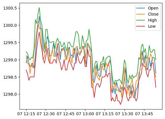
As shown above, column 'high' shows the highest price that it has reached at the given time and the column 'low' shows the the opposite. While the high and low prices should be useful when using other models, but as of now, we will just stick to using only the close price.
def plot_gold_sp_ftse(data, title):
    data['Datetime'] = pd.to_datetime(
        data['Date'] + ' ' + data['Time'],
        format='%d/%m/%Y %H:%M:%S'
    )

    plt.plot(data['Datetime'], data['Close'])
    plt.title(title)
    plt.show()

plt.rcParams['figure.figsize'] = [7, 5]
plot_gold_sp_ftse(gold_data, 'Gold')
plot_gold_sp_ftse(sp500_data, 'S&P 500')
plot_gold_sp_ftse(ftse_data, 'FTSE')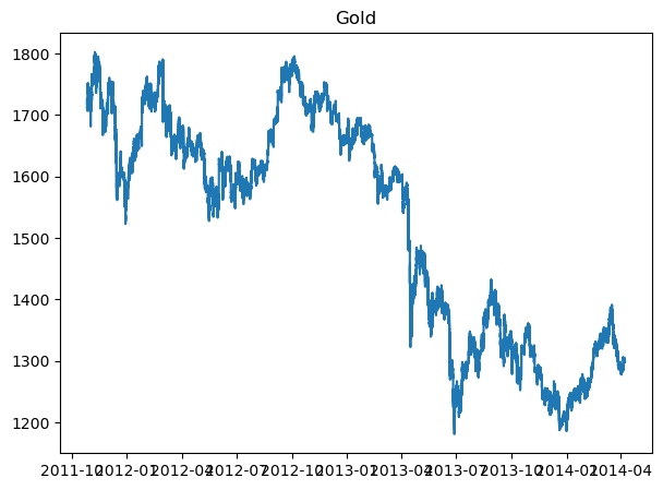
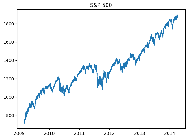
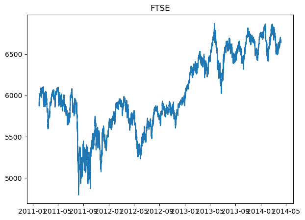
The above are the normal graphs for
-
Gold price, from Oct 2011 - Apr 2014
-
S&P500 price, from Nov 2009 - Apr 2014
-
FTSE price, from Feb 2011 - Apr 2014.
We will try to see if we can explore the relationship between them. Because just in a quick glance, we can see that Gold and S&P500 are inversely related, while FTSE is somewhat correlate to S&P500.
USDCUSDT Dataset
Next we will be looking into the USDCUSDT Dataset.
After using both methods, it seems to be quite quite undetermined.
usdcusdt_data = pd.read_csv('Datasets/USDC-USDT.csv')

usdcusdt_data.head()| Unnamed: 0 | unix | date | symbol | open | high | low | close | Volume USDC | Volume USDT | tradecount |
|---|---|---|---|---|---|---|---|---|---|---|
| 0 | 1635552000000 | 2021-10-30 00:00:00 | USDC/USDT | 1 | 1 | 0.9999 | 0.9999 | 740710 | 740678 | 277 |
| 1 | 1635465600000 | 2021-10-29 00:00:00 | USDC/USDT | 0.9995 | 1 | 0.9994 | 1 | 1.46553e+08 | 1.46532e+08 | 43366 |
| 2 | 1635379200000 | 2021-10-28 00:00:00 | USDC/USDT | 0.9994 | 0.9997 | 0.999 | 0.9995 | 2.97686e+08 | 2.97482e+08 | 58314 |
| 3 | 1635292800000 | 2021-10-27 00:00:00 | USDC/USDT | 0.9997 | 1 | 0.9976 | 0.9994 | 2.93017e+08 | 2.92868e+08 | 67437 |
| 4 | 1635206400000 | 2021-10-26 00:00:00 | USDC/USDT | 1.0003 | 1.0008 | 0.9993 | 0.9998 | 2.10106e+08 | 2.10147e+08 | 56204 |
usdcusdt_data['date']0 2021-10-30 00:00:00
1 2021-10-29 00:00:00
2 2021-10-28 00:00:00
3 2021-10-27 00:00:00
4 2021-10-26 00:00:00
...
1046 2018-12-19 00:00:00
1047 2018-12-18 00:00:00
1048 2018-12-17 00:00:00
1049 2018-12-16 00:00:00
1050 2018-12-15 00:00:00
Name: date, Length: 1051, dtype: objectusdcusdt_data.describe()| Unnamed: 0 | unix | open | high | low | close | Volume USDC | Volume USDT | tradecount |
|---|---|---|---|---|---|---|---|---|
| count | 1051 | 1051 | 1051 | 1051 | 1051 | 1051 | 1051 | 1051 |
| mean | 1.59019e+12 | 1.00001 | 1.011 | 0.998193 | 0.999991 | 5.50997e+07 | 5.50802e+07 | 29534.8 |
| std | 2.6226e+10 | 0.003651 | 0.281 | 0.004549 | 0.003629 | 7.75637e+07 | 7.75237e+07 | 21174.2 |
| min | 1.54483e+12 | 0.987 | 0.9918 | 0.9367 | 0.9866 | 542413 | 548254 | 277 |
| 25% | 1.56751e+12 | 0.999 | 1 | 0.9975 | 0.999 | 7.135e+06 | 7.13665e+06 | 14527 |
| 50% | 1.59019e+12 | 0.9997 | 1.0006 | 0.999 | 0.9997 | 1.47944e+07 | 1.47597e+07 | 24644 |
| 75% | 1.61287e+12 | 1.0003 | 1.0022 | 0.9997 | 1.0003 | 9.38658e+07 | 9.38618e+07 | 39083 |
| max | 1.63555e+12 | 1.0318 | 10.11 | 1.0238 | 1.0318 | 7.76166e+08 | 7.75546e+08 | 196022 |
Based on the data descriptions above, we can see that unix and date can be used for the datetime column, as both of the columns provide datetime information. Symbol column would not be useful in this context, among the price columns, we will be using the close price. As for the volume USDC, volume USDT, and tradecount, they will definitely benefit with other models, but we can explore how they look when we were to plot them
usdcusdt_explore_columns = ['close', 'Volume USDC', 'Volume USDT', 'tradecount']
usdcusdt_data['date'] = pd.to_datetime(usdcusdt_data['date'])

for column in usdcusdt_explore_columns:
    plt.plot(usdcusdt_data['date'], usdcusdt_data[column])
    plt.title(column)
    plt.show()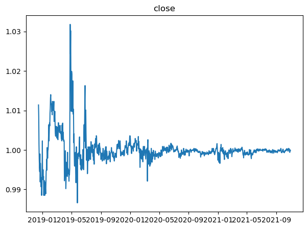

With them visualized, we can easily pick them to perform any form of analysis when required.
We can observe that the 'close' price column that at the start, the data has very high variance but exponentially decrease in its volatility, but the mean of the data might be the same overall.
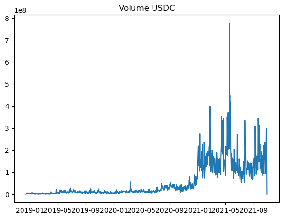
For the volume, both had very low amounts and then increased. It can be seen that the entire portion of the graph shifted upwards with the mean.
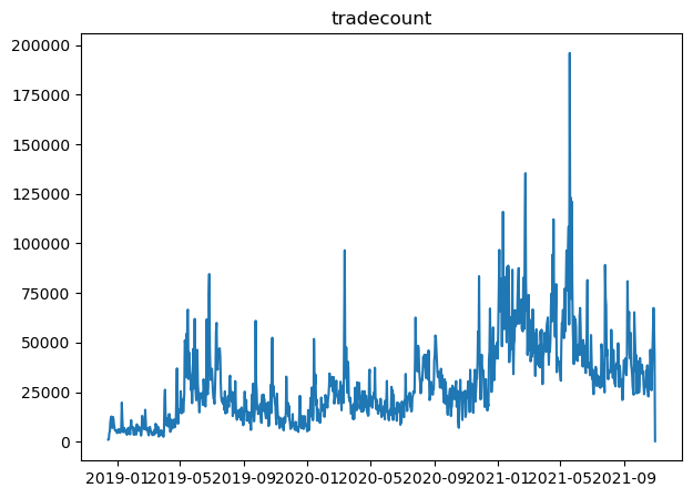
Tradecount column data seem to have some seasonality to it, with some form of repeating waves.
Cinema Ticket Dataset
While this dataset consists of time component and it is time series, it is not directly apparent. This is because the dataset not only includes a datetime information, but also status of the ticket sale of the specific cinema. Therefore, we will need to first do some pre-processing.
cinemaTicket_data = pd.read_csv('Datasets/cinemaTicket_Ref.csv')

cinemaTicket_data.head()| Unnamed: 0 | film_code | cinema_code | total_sales | tickets_sold | tickets_out | show_time | occu_perc | ticket_price | ticket_use | capacity | date | month | quarter | day |
|---|---|---|---|---|---|---|---|---|---|---|---|---|---|---|
| 0 | 1492 | 304 | 3900000 | 26 | 0 | 4 | 4.26 | 150000 | 26 | 610.329 | 2018-05-05 | 5 | 2 | 5 |
| 1 | 1492 | 352 | 3360000 | 42 | 0 | 5 | 8.08 | 80000 | 42 | 519.802 | 2018-05-05 | 5 | 2 | 5 |
| 2 | 1492 | 489 | 2560000 | 32 | 0 | 4 | 20 | 80000 | 32 | 160 | 2018-05-05 | 5 | 2 | 5 |
| 3 | 1492 | 429 | 1200000 | 12 | 0 | 1 | 11.01 | 100000 | 12 | 108.992 | 2018-05-05 | 5 | 2 | 5 |
| 4 | 1492 | 524 | 1200000 | 15 | 0 | 3 | 16.67 | 80000 | 15 | 89.982 | 2018-05-05 | 5 | 2 | 5 |
Let's say for this project, we would like t be able to predict when is the best time to increase teh discount, so that it can encourage ticket sales during off peak hours. We will first need to explore which columns to be using that can best represent our analysis.
cinemaTicket_data.columnsIndex(['film_code', 'cinema_code', 'total_sales', 'tickets_sold',
'tickets_out', 'show_time', 'occu_perc', 'ticket_price', 'ticket_use',
'capacity', 'date', 'month', 'quarter', 'day'],
dtype='object')cinemaTicket_data.describe()| Unnamed: 0 | film_code | cinema_code | total_sales | tickets_sold | tickets_out | show_time | occu_perc | ticket_price | ticket_use | capacity | month | quarter | day |
|---|---|---|---|---|---|---|---|---|---|---|---|---|---|
| count | 142524 | 142524 | 142524 | 142524 | 142524 | 142524 | 142399 | 142524 | 142524 | 142399 | 142524 | 142524 | 142524 |
| mean | 1518.99 | 320.378 | 1.23473e+07 | 140.138 | 0.237413 | 3.9321 | 19.966 | 81234.6 | 139.9 | 854.724 | 6.77685 | 2.63472 | 16.1126 |
| std | 36.1844 | 159.701 | 3.06549e+07 | 279.759 | 2.92321 | 3.05628 | 22.6534 | 33236.6 | 279.565 | 953.118 | 2.19584 | 0.809692 | 8.94947 |
| min | 1471 | 32 | 20000 | 1 | 0 | 1 | 0 | 483.871 | -219 | -2 | 2 | 1 | 1 |
| 25% | 1485 | 181 | 1.26e+06 | 18 | 0 | 2 | 3.75 | 60000 | 18 | 276.994 | 5 | 2 | 8 |
| 50% | 1498 | 324 | 3.72e+06 | 50 | 0 | 3 | 10.35 | 79454.2 | 50 | 525.714 | 7 | 3 | 16 |
| 75% | 1556 | 474 | 1.11e+07 | 143 | 0 | 5 | 28.21 | 100000 | 143 | 1038.96 | 9 | 3 | 24 |
| max | 1589 | 637 | 1.26282e+09 | 8499 | 311 | 60 | 147.5 | 700000 | 8499 | 9692.1 | 11 | 4 | 31 |
When inspecting the columns, the .head() and .describe() output, we noted that there are film code identified, as well as cinema_code. While these details might be useful for other analysis, we might just explore ticket_sold, to which should be good enough to indicate the performance of a given cinema. Because there also got a date column, we can use it as the datetime column. There are also other time related columns, like month, quarter, and day. However, similar justification that it might be useful for other analysis, but for this project will use only the date column and ticket sold.
Then, it is also further noted that because there is cinema codes, identifying the cinema, let's explore this aspect.
cinemaTicket_data['Datetime'] = pd.to_datetime(cinemaTicket_data['date'])
cinemaTicket_data| Unnamed: 0 | film_code | cinema_code | total_sales | tickets_sold | tickets_out | show_time | occu_perc | ticket_price | ticket_use | capacity | date | month | quarter | day | Datetime |
|---|---|---|---|---|---|---|---|---|---|---|---|---|---|---|---|
| 0 | 1492 | 304 | 3900000 | 26 | 0 | 4 | 4.26 | 150000.0 | 26 | 610.328638 | 2018-05-05 | 5 | 2 | 5 | 2018-05-05 |
| 1 | 1492 | 352 | 3360000 | 42 | 0 | 5 | 8.08 | 80000.0 | 42 | 519.801980 | 2018-05-05 | 5 | 2 | 5 | 2018-05-05 |
| 2 | 1492 | 489 | 2560000 | 32 | 0 | 4 | 20.00 | 80000.0 | 32 | 160.000000 | 2018-05-05 | 5 | 2 | 5 | 2018-05-05 |
| 3 | 1492 | 429 | 1200000 | 12 | 0 | 1 | 11.01 | 100000.0 | 12 | 108.991826 | 2018-05-05 | 5 | 2 | 5 | 2018-05-05 |
| 4 | 1492 | 524 | 1200000 | 15 | 0 | 3 | 16.67 | 80000.0 | 15 | 89.982004 | 2018-05-05 | 5 | 2 | 5 | 2018-05-05 |
| ... | ... | ... | ... | ... | ... | ... | ... | ... | ... | ... | ... | ... | ... | ... | ... |
| 142519 | 1569 | 495 | 1320000 | 22 | 0 | 2 | 3.86 | 60000.0 | 22 | 569.948187 | 2018-11-04 | 11 | 4 | 4 | 2018-11-04 |
| 142520 | 1569 | 474 | 1200000 | 15 | 0 | 1 | 65.22 | 80000.0 | 15 | 22.999080 | 2018-11-04 | 11 | 4 | 4 | 2018-11-04 |
| 142521 | 1569 | 524 | 1060000 | 8 | 0 | 3 | 9.20 | 132500.0 | 8 | 86.956522 | 2018-11-04 | 11 | 4 | 4 | 2018-11-04 |
| 142522 | 1569 | 529 | 600000 | 5 | 0 | 2 | 5.00 | 120000.0 | 5 | 100.000000 | 2018-11-04 | 11 | 4 | 4 | 2018-11-04 |
| 142523 | 1569 | 486 | 250000 | 5 | 0 | 1 | 1.79 | 50000.0 | 5 | 279.329609 | 2018-11-04 | 11 | 4 | 4 | 2018-11-04 |
cinemaTicket_data['show_time'].plot()
cinemaTicket_data['show_time'].hist()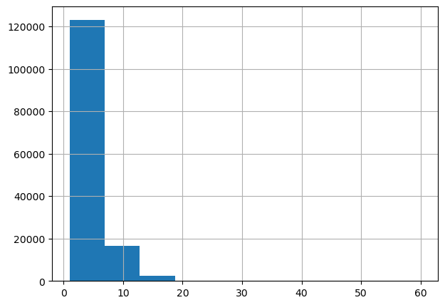
After checking the column showtime, we cannot conclude what does the column represent. At first glance, we might be able to use it to indicate the hours in datetime, and we might even be able to dig into finding out the hours that have lower sales. However, that would not be the case and we would look only into which day has the highest and lowest sale, and see if we are able to identify any trends overall.
# list of unique cinema
unique_cinemas = cinemaTicket_data['cinema_code'].unique()
unique_cinemas
array([304, 352, 489, 429, 524, 71, 163, 450, 51, 522, 43, 529, 82,
344, 73, 485, 518, 448, 431, 72, 144, 456, 238, 312, 168, 254,
214, 474, 445, 300, 362, 324, 452, 291, 479, 210, 428, 277, 56,
253, 243, 39, 310, 201, 457, 191, 532, 167, 266, 204, 380, 169,
162, 506, 537, 513, 467, 509, 165, 262, 486, 198, 508, 222, 98,
230, 156, 181, 141, 528, 94, 350, 442, 556, 475, 142, 35, 89,
34, 225, 182, 396, 50, 61, 487, 88, 338, 417, 194, 57, 285,
187, 159, 184, 81, 207, 339, 326, 531, 505, 492, 299, 507, 316,
333, 172, 526, 414, 115, 468, 490, 441, 430, 472, 511, 480, 470,
496, 466, 381, 368, 498, 195, 546, 516, 425, 488, 535, 196, 453,
321, 152, 390, 166, 247, 454, 464, 499, 460, 251, 481, 315, 307,
120, 250, 533, 221, 248, 313, 164, 70, 180, 160, 495, 314, 415,
174, 259, 471, 245, 83, 91, 365, 359, 286, 64, 426, 237, 536,
397, 476, 503, 491, 517, 55, 170, 175, 62, 539, 541, 540, 484,
514, 548, 432, 501, 447, 186, 477, 331, 515, 48, 33, 185, 155,
455, 461, 534, 273, 504, 249, 52, 482, 323, 451, 341, 306, 413,
292, 463, 223, 497, 525, 427, 231, 519, 183, 32, 553, 271, 276,
154, 521, 502, 402, 158, 473, 465, 561, 328, 558, 562, 424, 512,
560, 458, 637, 520, 557, 555, 543, 542, 565, 215, 376, 566],
dtype=int64)plt.rcParams['figure.figsize'] = [20, 12]
for cinema in unique_cinemas:
temp = cinemaTicket_data[cinemaTicket_data['cinema_code'] == cinema]
temp = temp[['Datetime','tickets_sold']]
temp = temp.groupby(['Datetime']).sum()
plt.plot(temp.index,temp['tickets_sold'])
# the legend list will be too long
# plt.legend(unique_cinemas)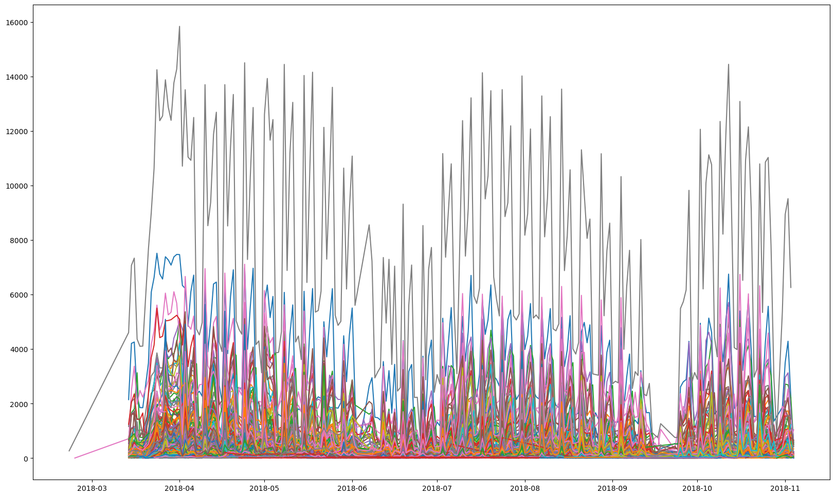
By getting the total sale at the given day for each cinema, and then plotting it, does not seem like a good idea, especially since because they have varying number of ticket sale.
However, we are able to note that there some form of repeatable patterns, trends or seasonality in the data. Let's use only 10 cinemas and plot it for visualization. Furthermore, later we shall look into take the average sales on a given day, and use that as the dataset moving forward for the cinema tickets dataset.
plt.rcParams['figure.figsize'] = [20, 12]

for cinema in unique_cinemas[:10]:

    temp = cinemaTicket_data[cinemaTicket_data['cinema_code'] == cinema]
    temp = temp[['Datetime','tickets_sold']]
    temp = temp.groupby(['Datetime']).sum()

    plt.plot(temp.index,temp['tickets_sold'],label=cinema)
    plt.legend()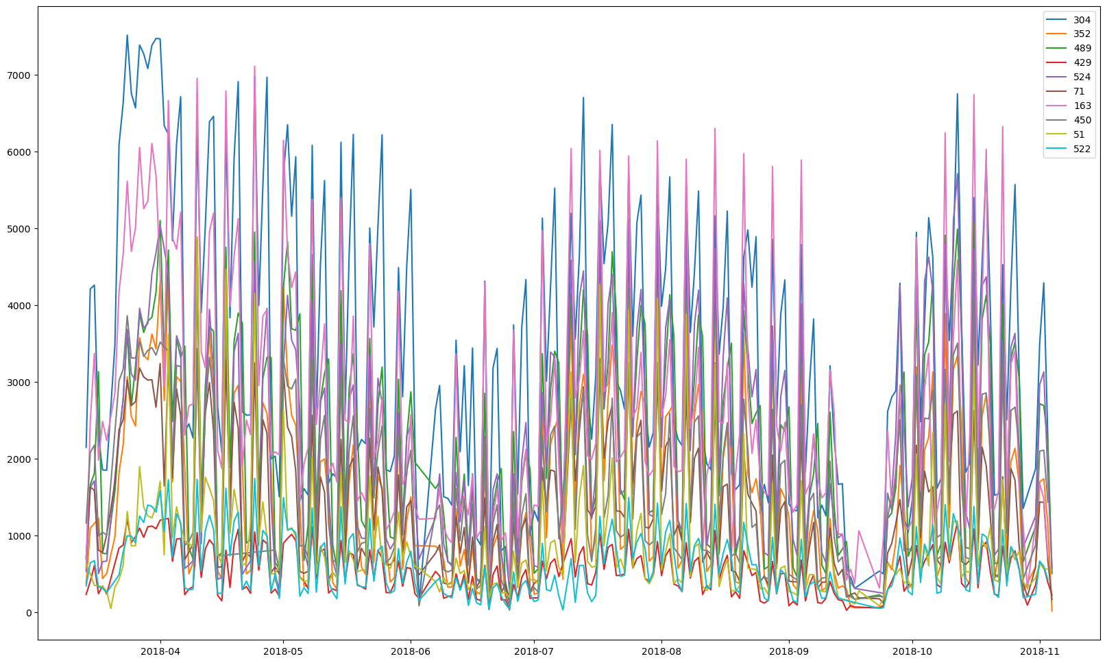
Using only 10 cinemas, the patterns are now more obvious.
ticketSales_data = cinemaTicket_data[['Datetime', 'tickets_sold']]
ticketSales_data = ticketSales_data.groupby('Datetime').mean()
ticketSales_data| ('Unnamed: 0_level_0', 'Datetime') | ('tickets_sold', 'Unnamed: 1_level_1') |
|---|---|
| 2018-02-21 | 267.000000 |
| 2018-02-23 | 3.000000 |
| 2018-03-14 | 125.650000 |
| 2018-03-15 | 178.675325 |
| 2018-03-16 | 175.461017 |
| ... | ... |
| 2018-10-31 | 70.583704 |
| 2018-11-01 | 113.653521 |
| 2018-11-02 | 126.824561 |
| 2018-11-03 | 75.431177 |
| 2018-11-04 | 49.894737 |
ticketSales_data.plot()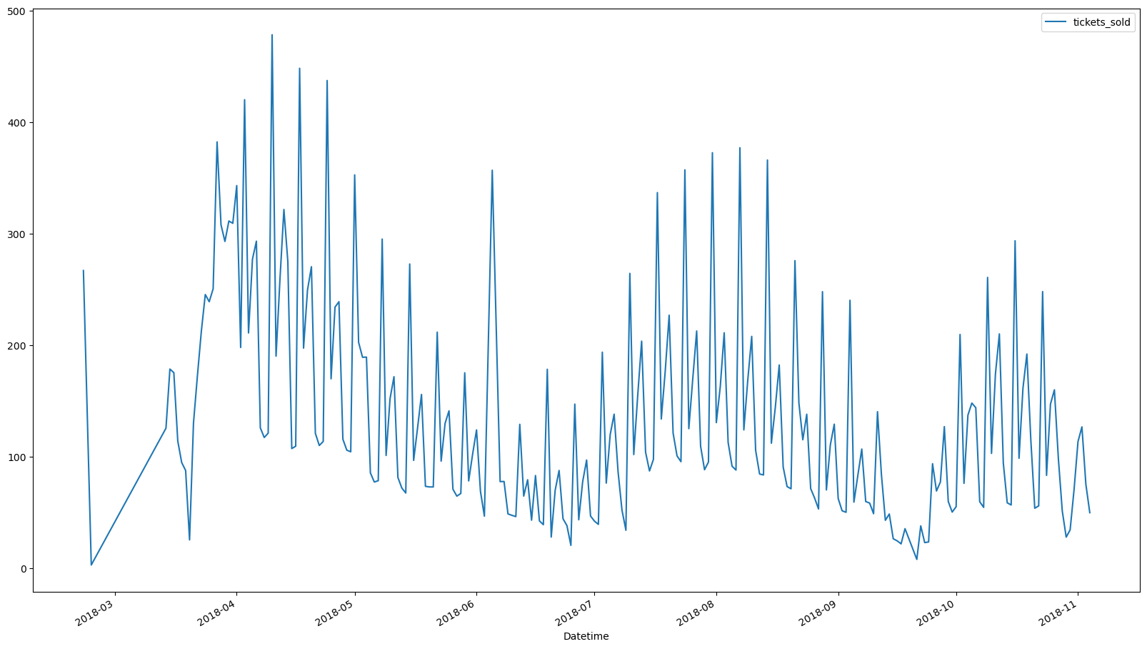
It seems that the first two entries are not properly maintained, or it could be outliers. Therefore, we would be dropping the first two entries.
ticketSales_data = ticketSales_data[2:]
ticketSales_data.plot()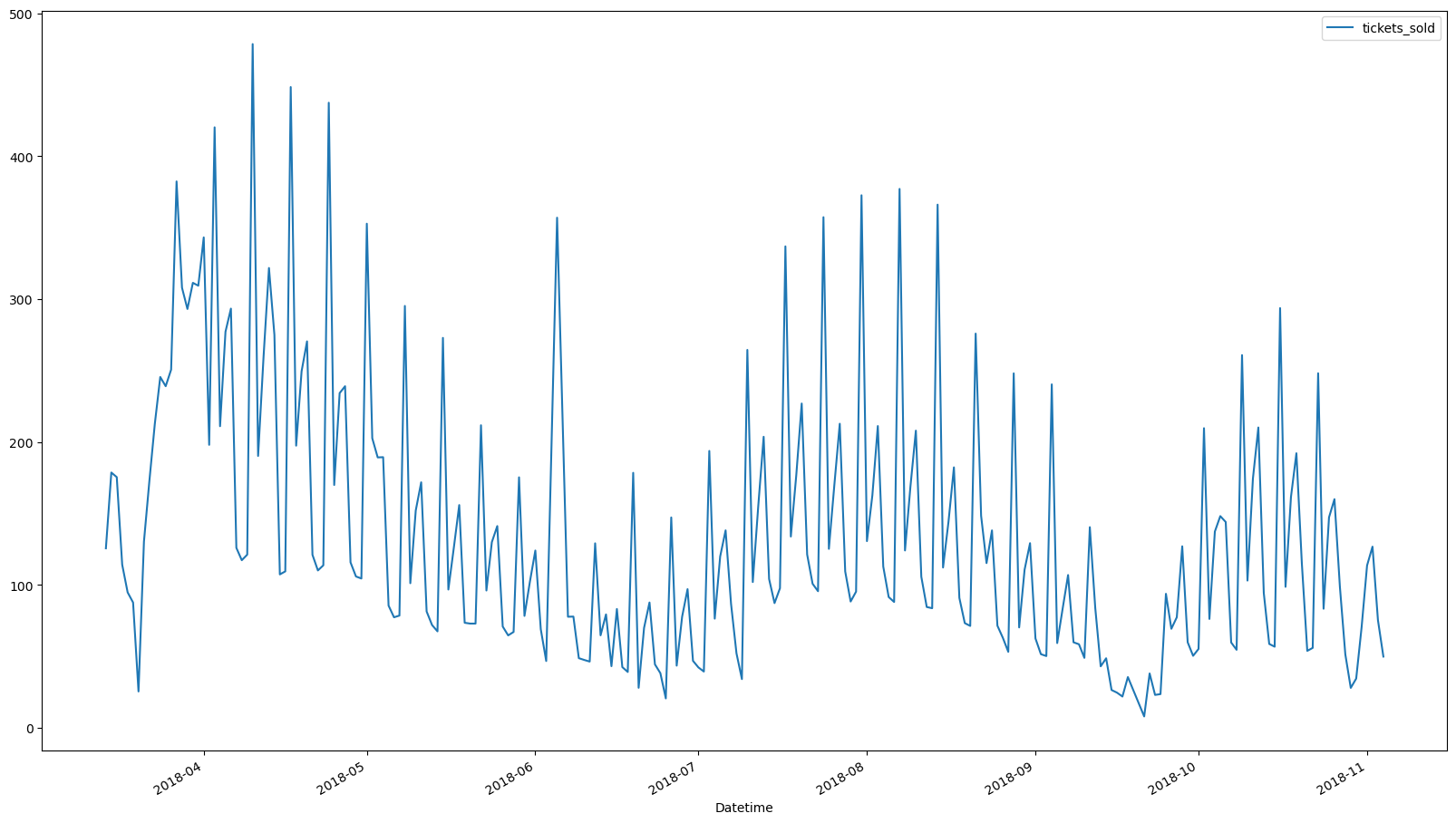
Stackoverflow Dataset
This dataset is a little more direct, where each columns signifies the topic that is being asked. For this project, we can look into the questions asked on the site overtime, from 2009 to 2019
mlStackoverflow_data = pd.read_csv('Datasets/MLTollsStackOverflow.csv')

mlStackoverflow_data.head()| Unnamed: 0 | month | nltk | spacy | stanford-nlp | python | r | numpy | scipy | matlab | machine-learning | ... | Plato | Sympy | Flair | stanford-nlp.1 | pyqt | Nolearn | Lasagne | OCR | Apache-spark-mlib | azure-virtual-machine |
|---|---|---|---|---|---|---|---|---|---|---|---|---|---|---|---|---|---|---|---|---|---|
| 0 | 09-Jan | 0 | 0 | 0 | 631 | 8 | 6 | 2 | 19 | 8 | ... | 0 | 1 | 0 | 0 | 5 | 0 | 0 | 5 | 0 | 0 |
| 1 | 09-Feb | 1 | 0 | 0 | 633 | 9 | 7 | 3 | 27 | 4 | ... | 0 | 0 | 0 | 0 | 5 | 0 | 0 | 11 | 0 | 0 |
| 2 | 09-Mar | 0 | 0 | 0 | 766 | 4 | 4 | 2 | 24 | 3 | ... | 0 | 0 | 0 | 0 | 7 | 0 | 0 | 2 | 0 | 0 |
| 3 | 09-Apr | 0 | 0 | 0 | 768 | 12 | 6 | 3 | 32 | 10 | ... | 0 | 0 | 0 | 0 | 11 | 0 | 0 | 5 | 0 | 0 |
| 4 | 09-May | 1 | 0 | 0 | 1003 | 2 | 7 | 2 | 42 | 7 | ... | 0 | 0 | 0 | 0 | 10 | 0 | 0 | 3 | 0 | 0 |
mlStackoverflow_data.columnsIndex(['month', 'nltk', 'spacy', 'stanford-nlp', 'python', 'r', 'numpy',
'scipy', 'matlab', 'machine-learning', 'pandas', 'pytorch', 'keras',
'nlp', 'apache-spark', 'hadoop', 'pyspark', 'python-3.x', 'tensorflow',
'deep-learning', 'neural-network', 'lstm', 'time-series', 'pillow',
'rasa', 'opencv', 'pipenv', 'seaborn', 'Dask', 'jupyter', 'AllenNLP',
'Theano', 'plotly', 'scikit-learn', 'BeautifulSoup', 'scrapy', 'Gensim',
'FastText', 'Pydot', 'Pybrain', 'Pytil', 'Pygame', 'Colab', 'Shogun',
'KNIME', 'Apache', 'Gunicorn', 'Pygtk', 'Weka', 'Conda', 'Ray',
'matlab.1', 'accord.net', 'regression', 'classification', 'correlation',
'cluster-analysis', 'H2o', 'Mallet', 'Numba', 'Tableau', 'Trifacta',
'PyArrow', 'Rasterio', 'Orange3', 'PyMC3', 'Opennn', 'Oryx', 'Istio',
'Venes', 'Plotnine', 'Gluon', 'Plato', 'Sympy', 'Flair',
'stanford-nlp.1', 'pyqt', 'Nolearn', 'Lasagne', 'OCR',
'Apache-spark-mlib', 'azure-virtual-machine'],
dtype='object')mlStackoverflow_data['month']0 09-Jan
1 09-Feb
2 09-Mar
3 09-Apr
4 09-May
...
127 19-Aug
128 19-Sep
129 19-Oct
130 19-Nov
131 19-Dec
Name: month, Length: 132, dtype: objectGiven that the topics of machine learning should have increase over the 10 years, especially with the recent explosion of interest for generative AI. We will see some relevant topics over the years.
mlStackoverflow_data['Datetime'] = pd.to_datetime(mlStackoverflow_data['month'], format='%y-%b')
mlStackoverflow_data.head()| Unnamed: 0 | month | nltk | spacy | stanford-nlp | python | r | numpy | scipy | matlab | machine-learning | ... | Sympy | Flair | stanford-nlp.1 | pyqt | Nolearn | Lasagne | OCR | Apache-spark-mlib | azure-virtual-machine | Datetime |
|---|---|---|---|---|---|---|---|---|---|---|---|---|---|---|---|---|---|---|---|---|---|
| 0 | 09-Jan | 0 | 0 | 0 | 631 | 8 | 6 | 2 | 19 | 8 | ... | 1 | 0 | 0 | 5 | 0 | 0 | 5 | 0 | 0 | 2009-01-01 |
| 1 | 09-Feb | 1 | 0 | 0 | 633 | 9 | 7 | 3 | 27 | 4 | ... | 0 | 0 | 0 | 5 | 0 | 0 | 11 | 0 | 0 | 2009-02-01 |
| 2 | 09-Mar | 0 | 0 | 0 | 766 | 4 | 4 | 2 | 24 | 3 | ... | 0 | 0 | 0 | 7 | 0 | 0 | 2 | 0 | 0 | 2009-03-01 |
| 3 | 09-Apr | 0 | 0 | 0 | 768 | 12 | 6 | 3 | 32 | 10 | ... | 0 | 0 | 0 | 11 | 0 | 0 | 5 | 0 | 0 | 2009-04-01 |
| 4 | 09-May | 1 | 0 | 0 | 1003 | 2 | 7 | 2 | 42 | 7 | ... | 0 | 0 | 0 | 10 | 0 | 0 | 3 | 0 | 0 | 2009-05-01 |
relevant_topics = ['python', 'machine-learning', 'deep-learning', 'time-series', 'regression', 'pytorch', 'tensorflow', 'classification']

plt.rcParams['figure.figsize'] = [7,5]

for topic in relevant_topics:
    plt.plot(mlStackoverflow_data['Datetime'], mlStackoverflow_data[topic])
    plt.scatter(mlStackoverflow_data['Datetime'], mlStackoverflow_data[topic], s=10)
    plt.title(topic)
    plt.show()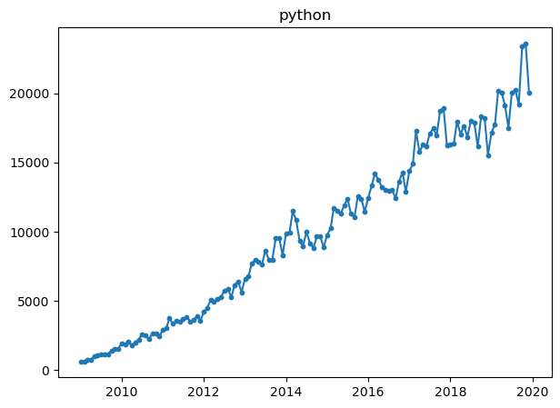
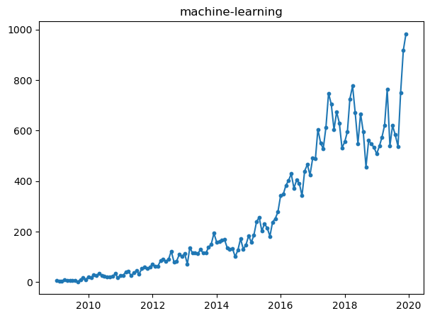
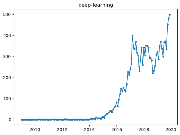
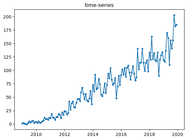
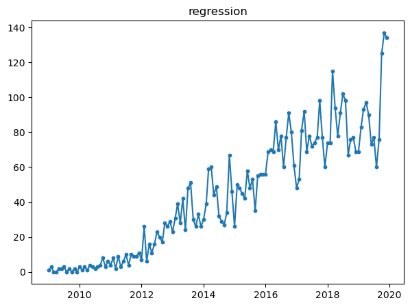
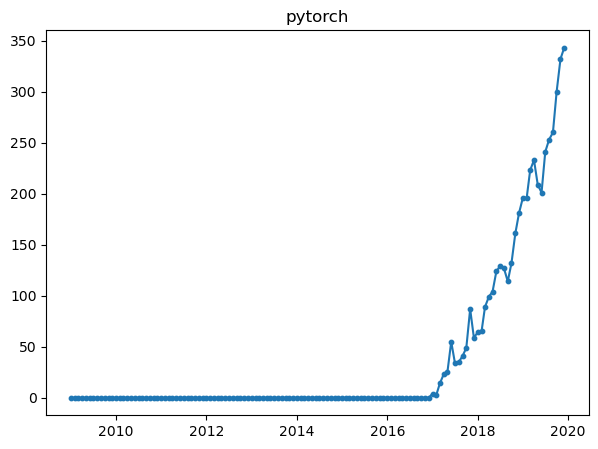
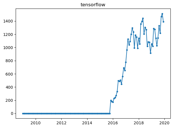
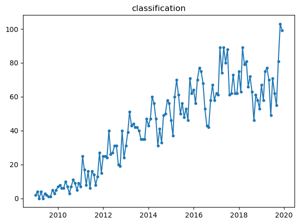
All of them, shows different properties in the graph. For example, while pytorch and tensorflow had beginnings around 2016, but they seem to increase a lot when observing the slope.
Multiplicative or Additive - Visual Identification
We will look into some dataset to see if there are multiplicative or additive. We will use the gold dataset, python and deep learning topic in the stackoverflow dataset and the cinema dataset to see if they are additive or multiplicative.
Based on the textbook that this course is based on, the difference between additive and multiplicative datsets are that one is the sum of seasonal component, trend component and residual component, and one is the product of all three. As shown in the equations below:
-
Additive:
-
Multiplicative:
Hence, to truly find out, we can decompose the time series into the components mentioned, seasonality, trend and residual.
However, based on the courses' lectures, it is also mentioned that we can identify based on the dispersion and shape of the differenced dataset, as shown below.
Gold Dataset - Close Price
gold_data['Close'].plot()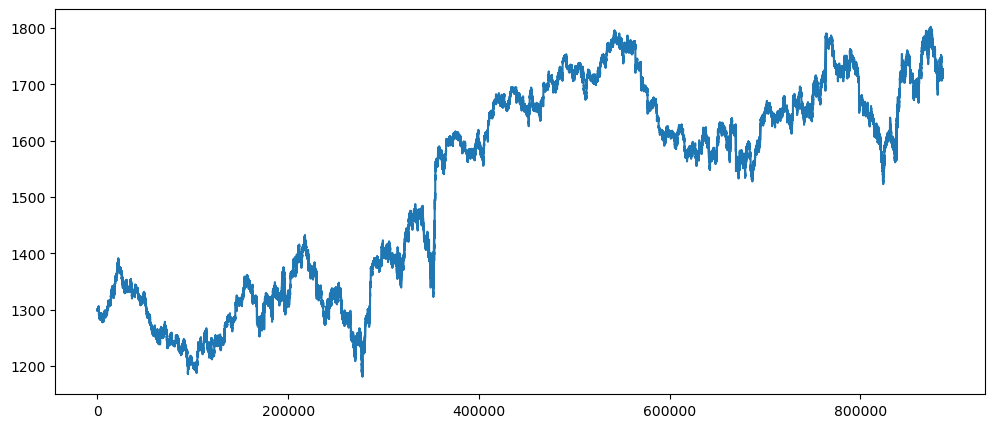
gold_data['Diff'] = gold_data['Close'] - gold_data['Close'].shift()
gold_data.plot.scatter(x = 'Close', y = 'Diff')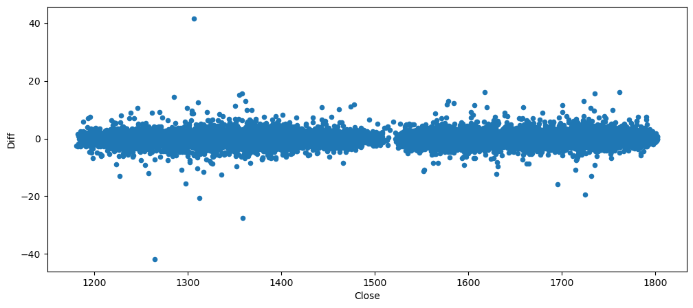
As observed, regardless or what value x, the y stays very consistent. Therefore, the changes between the price are not steep or drastic. Which represent an additive chart.
Stakeoverflow Dataset - Python
While the chart shows that it is linearly increase over time, when we check for additivity or multiplicity, turns out this is multiplicative, as shown in the scatter plot below. Where there are instance of x with very little change, while on the other end, the x values have higher change.
mlStackoverflow_data['python'].plot()
mlStackoverflow_data['python-diff'] = mlStackoverflow_data['python'] - mlStackoverflow_data['python'].shift()
mlStackoverflow_data.plot.scatter(x='python', y = 'python-diff')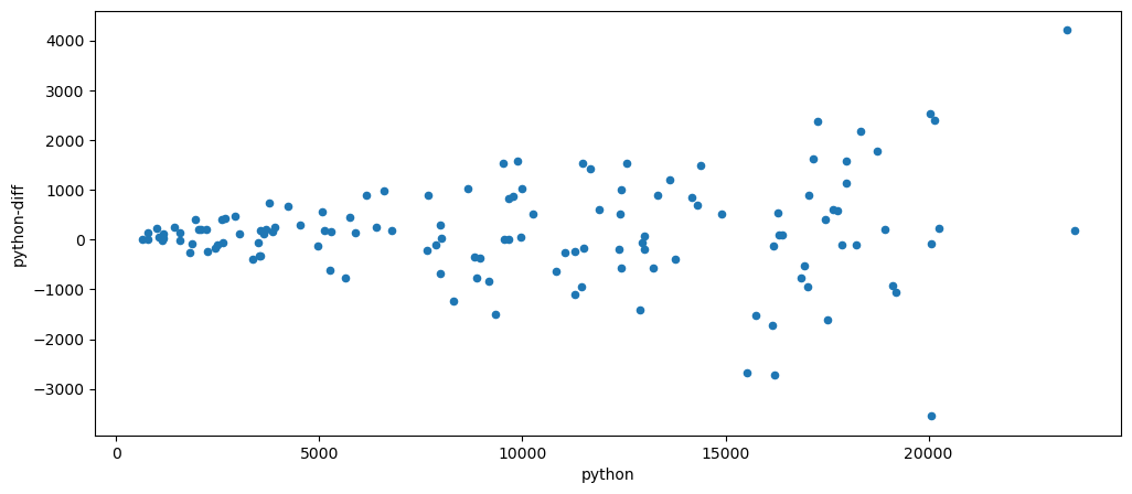
This is a multiplicative dataset because there is an obvious dispersion of y values, as x increases.
mlStackoverflow_data['logged_python'] = np.log(mlStackoverflow_data['python'])
mlStackoverflow_data['logged_python'].plot()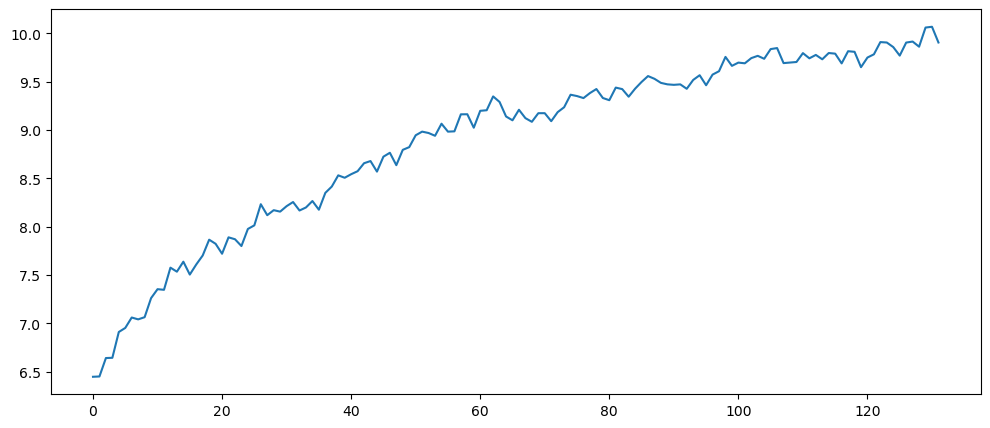
Even after logging, the chart still looks like it might be multiplicative.
mlStackoverflow_data['logged_python_diff'] = mlStackoverflow_data['logged_python'] - mlStackoverflow_data['logged_python'].shift()
mlStackoverflow_data.plot.scatter(x='logged_python', y='logged_python_diff')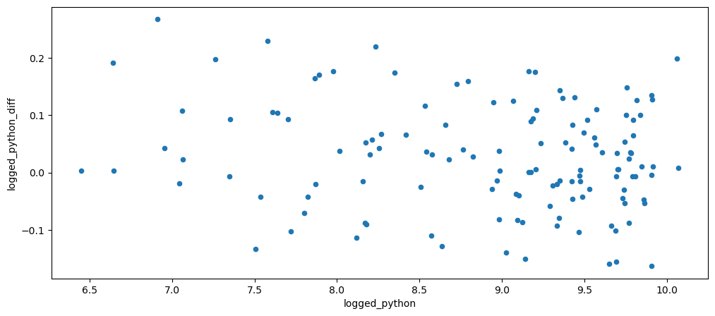
However, based on the result, the chart now looks more additive than it is multiplicative as the y values are now more consistent with the increase in x.
Stackoverflow Dataset - Machine Learning
Machine learning dataset was chosen because of its higher increase at the end of the chart. This shows that it is highly likely to be multiplicative.
mlStackoverflow_data['machine-learning'].plot()
mlStackoverflow_data['machine-learning-diff'] = mlStackoverflow_data['machine-learning'] - mlStackoverflow_data['machine-learning'].shift()
mlStackoverflow_data.plot.scatter(x='machine-learning', y='machine-learning-diff')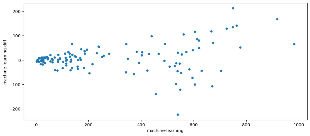
As guessed, it is a multiplicative chart.
mlStackoverflow_data['logged_ml'] = np.log(mlStackoverflow_data['machine-learning'])
mlStackoverflow_data['logged_ml'].plot()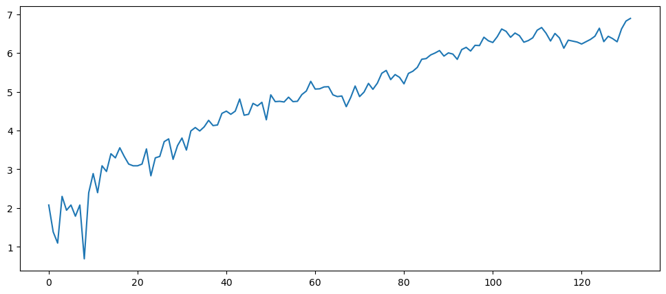
Now we shall explore the logged chart. Now the charts looks more linear, which leads more to additive.
mlStackoverflow_data['logged_ml_diff'] = mlStackoverflow_data['logged_ml'] - mlStackoverflow_data['logged_ml'].shift()
mlStackoverflow_data.plot.scatter(x='logged_ml', y='logged_ml_diff')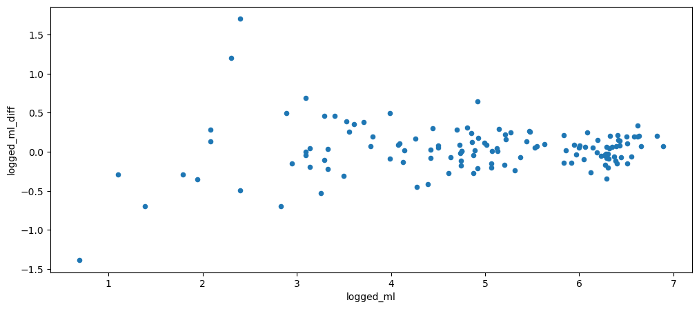
As shown, while there are still areas of higher dispersed y values, it is better than it was without logging.
Cinema Ticket Dataset - Tickets Sold
This dataset was chosen because out of curiously, a strong seasonal dataset, would be additive or multiplicative.
ticketSales_data['tickets_sold'].plot()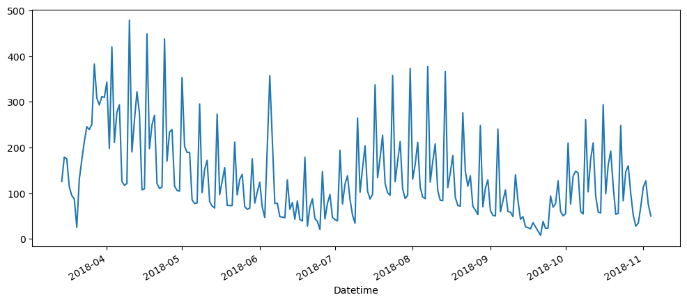
ticketSales_data['tickets_sold_diff'] = ticketSales_data['tickets_sold'] - ticketSales_data['tickets_sold'].shift()
ticketSales_data.plot.scatter(x='tickets_sold', y ='tickets_sold_diff')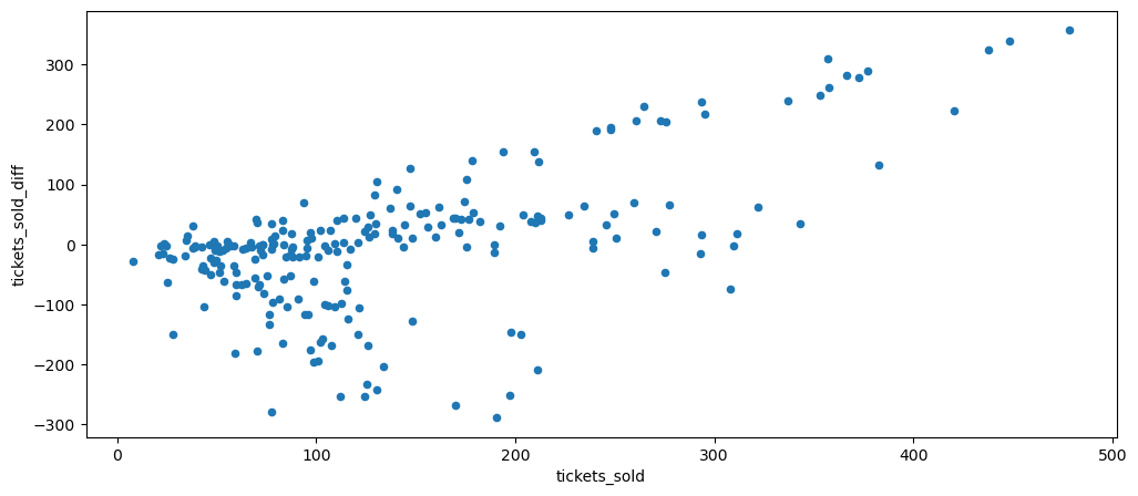
Based on the scatter plot, it seems like it is multiplicative, let's try logging it.
ticketSales_data['logged_sales'] = np.log(ticketSales_data['tickets_sold'])
ticketSales_data['logged_sales'].plot()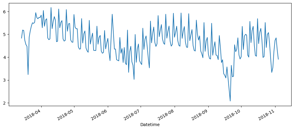
ticketSales_data['logged_sales_diff'] = ticketSales_data['logged_sales'] - ticketSales_data['logged_sales'].shift()
ticketSales_data.plot.scatter(x='logged_sales', y ='logged_sales_diff')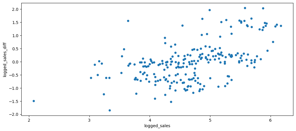
Based on the result, it looks like the multiplicity of has decreased and looks more additive with the values dispersed more consistently has compared to the one before.
Stationarity
See if any of data are stationary?
Visually, upon first glance, we can see that all of the current dataset, is not stationary, as most of them have some form trend, seasonality, varying means and variance. Therefore, let's implement ways to make them stationary and ensure that they are stationary. The dataset that we will be using is gold dataset and machine learning.
gold_data['Close'].plot()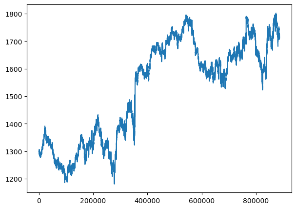
mlStackoverflow_data['machine-learning'].plot()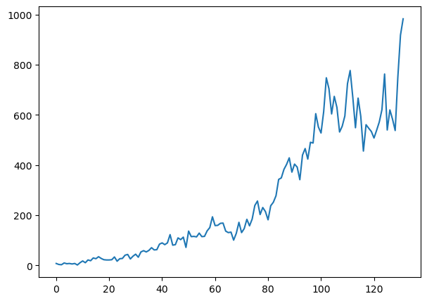
Random walk model or Simple Differencing
For many cases, just by finding the difference between the current period and previous period, should be enough to make the time-series data to be stationary.
gold_data['Close_Diffrenced'] = gold_data['Close'] - gold_data['Close'].shift()
gold_data['Close_Diffrenced'].plot()
mlStackoverflow_data['machine-learning_differenced'] = mlStackoverflow_data['machine-learning'] - mlStackoverflow_data['machine-learning'].shift()
mlStackoverflow_data['machine-learning_differenced'].plot()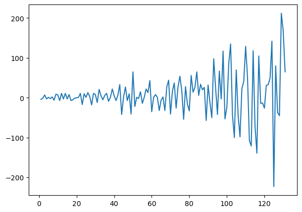
While we can visually see that both the graph has no more trend and has become more stationary than before, there are still some things to note. For the gold data, it is basically the ideal stationary data outcome, with some areas of outliers, but mostly, it is have a very steady mean and variance. However, even though we have use this method, the stackoverflow questions dataset still as an increase of variance overtime. Let's use some test to see if it is stationary or not. If not, we shall apply more differencing.
KPSS and ADF Test
We will be using the KPSS and ADF test to see if both of the above are stationary data.
from statsmodels.tsa.stattools import kpss

# Referred the below for the function and the use of kpss
# https://www.machinelearningplus.com/time-series/kpss-test-for-stationarity/

def kpss_test(series):
    statistic, p_value, n_lags, critical_values = kpss(series)
    print('KPSS Stat: ', statistic)
    print('p-value: ', p_value)
    print('Number of lags:', n_lags)
    print('Critial Values:')

    for key, value in critical_values.items():
        print(f'   {key} : {value}')
    print(f'Result: The series is {"not " if p_value < 0.05 else ""}stationary')

print('Gold Data-------------------')
print('=====Before Differencing:')
kpss_test(gold_data['Close'])
print()
print('=====After Differencing:')
kpss_test(gold_data['Close_Diffrenced'][1:])
Gold Data-------------------
=====Before Differencing:
KPSS Stat: 133.7235404045421
p-value: 0.01
Number of lags: 518
Critial Values:
10% : 0.347
5% : 0.463
2.5% : 0.574
1% : 0.739
Result: The series is not stationary
=====After Differencing:
KPSS Stat: 0.06604071713292024
p-value: 0.1
Number of lags: 44
Critial Values:
10% : 0.347
5% : 0.463
2.5% : 0.574
1% : 0.739
Result: The series is stationaryprint('StackOverFlow ML Data-------------------')
print('=====Before Differencing:')
kpss_test(mlStackoverflow_data['machine-learning'])
print()
print('=====After Differencing:')
kpss_test(mlStackoverflow_data['machine-learning_differenced'][1:])StackOverFlow ML Data-------------------
=====Before Differencing:
KPSS Stat: 1.8470519859412013
p-value: 0.01
Number of lags: 6
Critial Values:
10% : 0.347
5% : 0.463
2.5% : 0.574
1% : 0.739
Result: The series is not stationary
=====After Differencing:
KPSS Stat: 0.29869005236660856
p-value: 0.1
Number of lags: 10
Critial Values:
10% : 0.347
5% : 0.463
2.5% : 0.574
1% : 0.739
Result: The series is stationaryAccording to the KPSS test, even after the simple differencing for the the questions in stackoverflow, is enough to be stationary. Let's see for the adfuller test.
For the adfuller test, the closer the p-value it is to 0, the higher the likelihood for us to assume that there is no unit root in the time-series and that it is stationary. Assuming we were to use p-values of 0.05.
from statsmodels.tsa.stattools import adfuller

def adftest(series):
    res = adfuller(series)
    print('AdfTest Stat: ', res[0])
    print('p-value: ', res[1])
    print('Number of lags:', res[2])
    print('Number of observation:', res[3])
    print('Critial Values:')

    for key, value in res[4].items():
        print(f'   {key} : {value}')

    if res[1] < 0.05:
        print('The series is stationary')
    else:
        print('The series is not stationary')

adftest(mlStackoverflow_data['machine-learning'])
AdfTest Stat: 0.6666371271225812
p-value: 0.9891479891628309
Number of lags: 12
Number of observation: 119
Critial Values:
1% : -3.4865346059036564
5% : -2.8861509858476264
10% : -2.579896092790057
The series is not stationaryadftest(mlStackoverflow_data['machine-learning_differenced'][1:])AdfTest Stat: -2.054928456415778
p-value: 0.2630197887870384
Number of lags: 11
Number of observation: 119
Critial Values:
1% : -3.4865346059036564
5% : -2.8861509858476264
10% : -2.579896092790057
The series is not stationaryUsing the adfuller test, the simple differencing was not enough. While the p-values have dropped from 0.98 to 0.26, we can still try to make the dataset more stationary.
Second Order Differencing
firstDifference = mlStackoverflow_data['machine-learning'] - mlStackoverflow_data['machine-learning'].shift()

firstDifference
0 NaN
1 -4.0
2 -1.0
3 7.0
4 -3.0
...
127 -37.0
128 -45.0
129 212.0
130 168.0
131 65.0
Name: machine-learning, Length: 132, dtype: float64secondDifference = mlStackoverflow_data['machine-learning'].shift() - mlStackoverflow_data['machine-learning'].shift(2)
secondDifference0 NaN
1 NaN
2 -4.0
3 -1.0
4 7.0
...
127 80.0
128 -37.0
129 -45.0
130 212.0
131 168.0
Name: machine-learning, Length: 132, dtype: float64secondOrderDifference = firstDifference - secondDifference
secondOrderDifference0 NaN
1 NaN
2 3.0
3 8.0
4 -10.0
...
127 -117.0
128 -8.0
129 257.0
130 -44.0
131 -103.0
Name: machine-learning, Length: 132, dtype: float64plt.plot(firstDifference)
plt.plot(secondOrderDifference)
plt.show()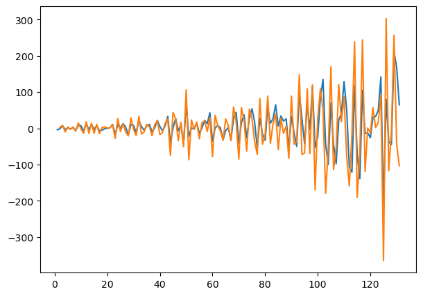
adftest(secondOrderDifference[2:])AdfTest Stat: -6.611299198025336
p-value: 6.367085815585583e-09
Number of lags: 10
Number of observation: 119
Critial Values:
1% : -3.4865346059036564
5% : -2.8861509858476264
10% : -2.579896092790057
The series is stationaryWe can see that visually, the difference between the simple difference and second order differencing, the second order differencing looked like the variance increased as we do see higher highs and lower low in the graph as compared to the simple differencing. The orange graph is the second order differencing. However, based on the adfuller test, it is stationary.
Seasonal Differencing
Seasonal differencing is based on the formula below, which is subtract by the current value with a value in the past
However, we will need to loop through some values to find this. Another method of seasonal differencing is to understand a season timeframe, then get the mean of each season, and apply subtraction according to respective season's mean.
lags = [3,5,10,20,50]

plt.rcParams['figure.figsize'] = [15,7]

for lag in lags:
    temp = mlStackoverflow_data['machine-learning'] - mlStackoverflow_data['machine-learning'].shift(lag)
    plt.plot(temp, label=str(lag) + " lag")

    print('Test for lag ' + str(lag) + "  =====================================")
    kpss_test(temp[lag:])
    print()
    adftest(temp[lag:])
    print()

plt.legend()
plt.show()Test for lag 3 =====================================
KPSS Stat: 0.2898885946621235
p-value: 0.1
Number of lags: 4
Critial Values:
10% : 0.347
5% : 0.463
2.5% : 0.574
1% : 0.739
Result: The series is stationary
AdfTest Stat: -2.25147303187454
p-value: 0.18809655506315798
Number of lags: 13
Number of observation: 115
Critial Values:
1% : -3.4885349695076844
5% : -2.887019521656941
10% : -2.5803597920604915
The series is not stationary
Test for lag 5 =====================================
KPSS Stat: 0.27908581626858614
p-value: 0.1
Number of lags: 4
Critial Values:
10% : 0.347
5% : 0.463
2.5% : 0.574
1% : 0.739
Result: The series is stationary
AdfTest Stat: -2.1942366663365926
p-value: 0.20834386047176706
Number of lags: 12
Number of observation: 114
Critial Values:
1% : -3.489057523907491
5% : -2.887246327182993
10% : -2.5804808802708528
The series is not stationary
Test for lag 10 =====================================
KPSS Stat: 0.35328244736991793
p-value: 0.09729204854744916
Number of lags: 5
Critial Values:
10% : 0.347
5% : 0.463
2.5% : 0.574
1% : 0.739
Result: The series is stationary
AdfTest Stat: -2.4158493770328726
p-value: 0.13731291632025688
Number of lags: 12
Number of observation: 109
Critial Values:
1% : -3.49181775886872
5% : -2.8884437992971588
10% : -2.5811201893779985
The series is not stationary
Test for lag 20 =====================================
KPSS Stat: 0.5230701441606662
p-value: 0.0364706882521022
Number of lags: 5
Critial Values:
10% : 0.347
5% : 0.463
2.5% : 0.574
1% : 0.739
Result: The series is not stationary
AdfTest Stat: -2.157009917873902
p-value: 0.2222165170167978
Number of lags: 12
Number of observation: 99
Critial Values:
1% : -3.498198082189098
5% : -2.891208211860468
10% : -2.5825959973472097
The series is not stationary
Test for lag 50 =====================================
KPSS Stat: 1.3102598299838486
p-value: 0.01
Number of lags: 5
Critial Values:
10% : 0.347
5% : 0.463
2.5% : 0.574
1% : 0.739
Result: The series is not stationary
AdfTest Stat: -0.5612811021960334
p-value: 0.8794931265993677
Number of lags: 12
Number of observation: 69
Critial Values:
1% : -3.528889992207215
5% : -2.9044395987933362
10% : -2.589655654274312
The series is not stationary
Surprisingly, the further you lag, does not mean that the data will become more stationary. As shown with the kpss and adfuller test, we can see that even using difference of lag 3, adfuller test already did not consider the time series as stationary. The KPSS result shows that from lag 20 onwards, the data is no longer stationary. We can also observed this because visually as the red and purple graph slowly becoming a upward trending graph.
Log and log differences
Let's see how does logging a time-series or getting the log differences, can effect the stationarity of a time-series. We will continue using the stackoverflow dataset on machine learning.
loggedMLtopic = np.log(mlStackoverflow_data['machine-learning'])
loggedMLtopic.plot()
It has made it into a trending time series, so now we can try apply simple differencing
differencedLoggedMLtopic = loggedMLtopic - loggedMLtopic.shift()
differencedLoggedMLtopic.plot()
kpss_test(differencedLoggedMLtopic[1:])KPSS Stat: 0.28055757025438893
p-value: 0.1
Number of lags: 55
Critial Values:
10% : 0.347
5% : 0.463
2.5% : 0.574
1% : 0.739
Result: The series is stationaryadftest(differencedLoggedMLtopic[1:])AdfTest Stat: -13.691197822513615
p-value: 1.342938733545792e-25
Number of lags: 1
Number of observation: 129
Critial Values:
1% : -3.482087964046026
5% : -2.8842185101614626
10% : -2.578864381347275
The series is stationaryBased on the both the test and visually, we have able to make the machine learning topic time series to be stationary.
Seasonality
Seasonality are data that has some form of repeating pattern and precipitability at a certain time frame.
Based on the current set of data we have, we can clearly see that the cinema dataset has repeatable pattern, very noticeable peak and trough. Therefore, we will look into this dataset for the seasonality adjustments.
Cinema Tickets
ticketSales_data.index.weekdayInt64Index([2, 3, 4, 5, 6, 0, 1, 2, 3, 4,
...
4, 5, 6, 0, 1, 2, 3, 4, 5, 6],
dtype='int64', name='Datetime', length=232)ticketSales_data.index.weekday.unique()Int64Index([2, 3, 4, 5, 6, 0, 1], dtype='int64', name='Datetime')ticketSales_data = ticketSales_data.assign(day=ticketSales_data.index.weekday)
ticketSales_data| ('Unnamed: 0_level_0', 'Datetime') | ('tickets_sold', 'Unnamed: 1_level_1') | ('day', 'Unnamed: 2_level_1') |
|---|---|---|
| 2018-03-14 | 125.650000 | 2 |
| 2018-03-15 | 178.675325 | 3 |
| 2018-03-16 | 175.461017 | 4 |
| 2018-03-17 | 114.192192 | 5 |
| 2018-03-18 | 94.831956 | 6 |
| ... | ... | ... |
| 2018-10-31 | 70.583704 | 2 |
| 2018-11-01 | 113.653521 | 3 |
| 2018-11-02 | 126.824561 | 4 |
| 2018-11-03 | 75.431177 | 5 |
| 2018-11-04 | 49.894737 | 6 |
# Because the timeframe in the dataset is not a full calendar year.
# Get the list of months that are involved
days = ticketSales_data.index.weekday.unique()
# Initializing season count and sum
seasonSum = [0] * len(days)
seasonCount = [0] * len(days)
for rowCount in range(len(ticketSales_data)):
currentValue, currentDay = ticketSales_data.iloc[rowCount,[0,1]]
seasonSum[int(currentDay)] += currentValue
seasonCount[int(currentDay)] += 1
print(seasonCount)
print(seasonSum)[32, 33, 32, 33, 34, 34, 34]
[2431.9228952621716, 8661.859799267784, 3712.1669864735404, 4930.762704784601, 5691.3748326994255, 3488.7014251378805, 2745.6502726189774]# Season Mean
seasonMean = [0] * len(days)
for count in range(len(seasonCount)):
seasonMean[count] = seasonSum[count] / seasonCount[count]
seasonMean[75.99759047694286,
262.48059997781166,
116.00521832729814,
149.4170516601394,
167.39337743233605,
102.60886544523179,
80.7544197829111]dataMean = np.mean(ticketSales_data['tickets_sold'].values)
dataMean136.47602981139818seasonOffsets = [x - dataMean for x in seasonMean]
seasonOffsets[-60.47843933445532,
126.00457016641349,
-20.47081148410004,
12.94102184874123,
30.917347620937875,
-33.86716436616639,
-55.72161002848708]adjustedTicketsSold = []
for count in range(len(ticketSales_data)):
currentValue, currentDay = ticketSales_data.iloc[count,[0,1]]
adjustedTicketsSold.append(currentValue - seasonOffsets[int(currentDay)])
adjustedTicketsSold[146.12081148410005,
165.73430282658344,
144.54366932821466,
148.0593565583586,
150.55356595135208,
...
91.05451518780374,
100.71249927801934,
95.90721378257089,
109.29834181226921,
105.61634687059234]ticketSales_data = ticketSales_data.assign(adjustedTicketSale = adjustedTicketsSold)
plt.rcParams['figure.figsize'] = [12, 5]
ticketSales_data.iloc[:, [0,2]].plot()
As we can observe, the orange plot is the adjusted ticket sales. The adjustment works because we can see that the peaks are now lower, while the trough are now higher generally. However, we are still able to note that there are still peaks and troughs even after the adjustment.
secondAdjustmentCount = [0] * len(days)
secondAdjustmentSum = [0] * len(days)
secondAdjustmentMean = [0] * len(days)
secondAdjustmentValue = []
for count in range(len(ticketSales_data)):
currentDay, currentValue = ticketSales_data.iloc[count, [1,2]]
secondAdjustmentCount[int(currentDay)] += 1
secondAdjustmentSum[int(currentDay)] += currentValue
print("Season Count:", secondAdjustmentCount)
print("Season Sum:", secondAdjustmentSum)
for count in range(len(secondAdjustmentSum)):
secondAdjustmentMean[count] = secondAdjustmentSum[count] / secondAdjustmentCount[count]
print("Season Mean:", secondAdjustmentMean)
secondMean = np.mean(ticketSales_data['adjustedTicketSale'].values)
print("Adjusted Ticket Sale Mean:", secondMean)
secondAdjustmentOffsets = [(x - secondMean) for x in secondAdjustmentMean]
print(secondAdjustmentOffsets)
secondAdjustedTickets = []
for count in range(len(ticketSales_data)):
currentValue, currentDay = ticketSales_data.iloc[count, [2,1]]
secondAdjustedTickets.append(currentValue - secondAdjustmentOffsets[int(currentDay)])
ticketSales_data = ticketSales_data.assign(second_adjusted_ticket_sales = secondAdjustedTickets)
plt.rcParams['figure.figsize'] = [12, 5]
ticketSales_data.iloc[:, [2,3]].plot()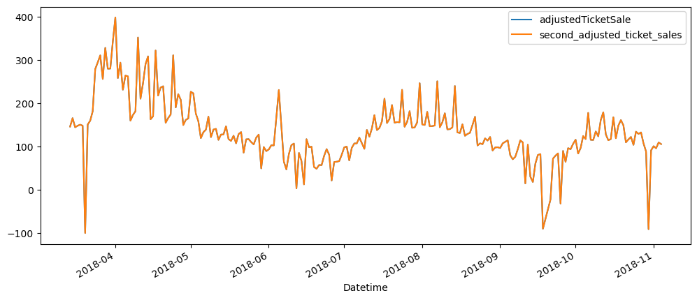
It is surprising to see that after the first adjustment, we are no longer able to remove more variances, lower the peaks and heighten the troughs, as the offsets list and the mean of the adjusted tickets sold column, are so close to each other.
weeks = ticketSales_data.index.week.unique()
weeksInt64Index([11, 12, 13, 14, 15, 16, 17, 18, 19, 20, 21, 22, 23, 24, 25, 26, 27,
28, 29, 30, 31, 32, 33, 34, 35, 36, 37, 38, 39, 40, 41, 42, 43,
44],
dtype='int64', name='Datetime')ticketSales_data = ticketSales_data.assign(week=ticketSales_data.index.isocalendar().week)
ticketSales_data| ('Unnamed: 0_level_0', 'Datetime') | ('tickets_sold', 'Unnamed: 1_level_1') | ('day', 'Unnamed: 2_level_1') | ('adjustedTicketSale', 'Unnamed: 3_level_1') | ('second_adjusted_ticket_sales', 'Unnamed: 4_level_1') | ('week', 'Unnamed: 5_level_1') |
|---|---|---|---|---|---|
| 2018-03-14 | 125.650000 | 2 | 146.120811 | 146.120811 | 11 |
| 2018-03-15 | 178.675325 | 3 | 165.734303 | 165.734303 | 11 |
| 2018-03-16 | 175.461017 | 4 | 144.543669 | 144.543669 | 11 |
| 2018-03-17 | 114.192192 | 5 | 148.059357 | 148.059357 | 11 |
| 2018-03-18 | 94.831956 | 6 | 150.553566 | 150.553566 | 11 |
| ... | ... | ... | ... | ... | ... |
| 2018-10-31 | 70.583704 | 2 | 91.054515 | 91.054515 | 44 |
| 2018-11-01 | 113.653521 | 3 | 100.712499 | 100.712499 | 44 |
| 2018-11-02 | 126.824561 | 4 | 95.907214 | 95.907214 | 44 |
| 2018-11-03 | 75.431177 | 5 | 109.298342 | 109.298342 | 44 |
| 2018-11-04 | 49.894737 | 6 | 105.616347 | 105.616347 | 44 |
weekAdjustmentCount = [0] * len(weeks)
weekAdjustmentSum = [0] * len(weeks)
weekAdjustmentMean = [0] * len(weeks)
weekAdjustmentValue = []
for count in range(len(ticketSales_data)):
currentWeek, currentValue = ticketSales_data.iloc[count, [4,0]]
weekAdjustmentCount[int(currentWeek)-11] += 1
weekAdjustmentSum[int(currentWeek)-11] += currentValue
print("Season Count:", weekAdjustmentCount)
print("Season Sum:", weekAdjustmentSum)
for count in range(len(weekAdjustmentSum)):
weekAdjustmentMean[count] = weekAdjustmentSum[count] / weekAdjustmentCount[count]
print("Season Mean:", weekAdjustmentMean)
weekMean = np.mean(ticketSales_data['adjustedTicketSale'].values)
print("Adjusted Ticket Sale Mean:", secondMean)
weekAdjustmentOffsets = [(x - weekMean) for x in weekAdjustmentMean]
print(weekAdjustmentOffsets)
weekAdjustedTickets = []
for count in range(len(ticketSales_data)):
currentWeek, currentValue = ticketSales_data.iloc[count, [4,0]]
weekAdjustedTickets.append(currentValue - weekAdjustmentOffsets[int(currentWeek)-11])
ticketSales_data = ticketSales_data.assign(week_adjusted_ticket_sales = weekAdjustedTickets)
plt.rcParams['figure.figsize'] = [12, 5]
ticketSales_data[['tickets_sold','week_adjusted_ticket_sales']].plot()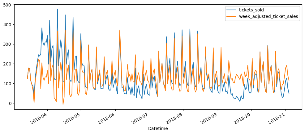
plt.rcParams['figure.figsize'] = [12, 5]
ticketSales_data[['tickets_sold','week_adjusted_ticket_sales','adjustedTicketSale']].plot()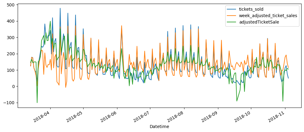
As it can be seen, the seasonality was more removed when we are using the day of the week trying adjust according to the mean of each day, rather than the mean of each week. The week adjusted ticket sales seem to more stationary, but the peaks and trough, while decreased, they are still very prominent. Hence, seasonality is still there.
USDCUSDT Tradecount
We can also explore on the USDCUSDT tradecount column which seem to look like that there are seasonality. We will applied the same steps as above.
for no, column in enumerate(usdcusdt_data.columns):
print(str(no) + " " + column)0 unix
1 date
2 symbol
3 open
4 high
5 low
6 close
7 Volume USDC
8 Volume USDT
9 tradecountusdcusdt_data.iloc[2,1].weekday()3usdcusdtDayAdjustmentCount = [0] * 31
usdcusdtDayWeekAdjustmentCount = [0] * 7
usdusdtMonthAdjustmentCount = [0] * 12
usdcusdtDayAdjustmentSum = [0] * 31
usdcusdtDayWeekAdjustmentSum = [0] * 7
usdcusdtMonthAdjustmentSum = [0] * 12
usdcusdtDayAdjustmentMean = [0] * 31
usdcusdtDayWeekAdjustmentMean = [0] * 7
usdcusdtMonthAdjustmentMean = [0] * 12
usdcusdtCloseMean = usdcusdt_data['tradecount'].mean()
for rowCount in range(len(usdcusdt_data)):
usdcusdtDayAdjustmentCount[usdcusdt_data.iloc[rowCount, 1].day-1] += 1
usdcusdtDayAdjustmentSum[usdcusdt_data.iloc[rowCount, 1].day-1] += usdcusdt_data.iloc[rowCount, 9]
usdcusdtDayWeekAdjustmentCount[usdcusdt_data.iloc[rowCount, 1].weekday()] += 1
usdcusdtDayWeekAdjustmentSum[usdcusdt_data.iloc[rowCount, 1].weekday()] += usdcusdt_data.iloc[rowCount, 9]
usdusdtMonthAdjustmentCount[usdcusdt_data.iloc[rowCount, 1].month-1] += 1
usdcusdtMonthAdjustmentSum[usdcusdt_data.iloc[rowCount, 1].month-1] += usdcusdt_data.iloc[rowCount, 9]
for count in range(len(usdcusdtDayAdjustmentSum)):
usdcusdtDayAdjustmentMean[count] = usdcusdtDayAdjustmentSum[count] / usdcusdtDayAdjustmentCount[count]
for count in range(len(usdcusdtDayWeekAdjustmentSum)):
usdcusdtDayWeekAdjustmentMean[count] = usdcusdtDayWeekAdjustmentSum[count] / usdcusdtDayWeekAdjustmentCount[count]
for count in range(len(usdcusdtMonthAdjustmentSum)):
usdcusdtMonthAdjustmentMean[count] = usdcusdtMonthAdjustmentSum[count] / usdusdtMonthAdjustmentCount[count]
dayAdjustmentOffset = [(x - usdcusdtCloseMean) for x in usdcusdtDayAdjustmentMean]
dayWeekAdjustmentOffset = [(x - usdcusdtCloseMean) for x in usdcusdtDayWeekAdjustmentMean]
monthAdjustmentOffset = [(x - usdcusdtCloseMean) for x in usdcusdtMonthAdjustmentMean]
dayAdjustedClose = []
dayWeekAdjustedClose = []
monthAdjustedClose = []
for rowCount in range(len(usdcusdt_data)):
currentValue, currentDatetime = usdcusdt_data.iloc[rowCount, [9,1]]
dayAdjustedClose.append(currentValue - dayAdjustmentOffset[currentDatetime.day - 1])
dayWeekAdjustedClose.append(currentValue - dayWeekAdjustmentOffset[currentDatetime.weekday()])
monthAdjustedClose.append(currentValue - monthAdjustmentOffset[currentDatetime.month - 1])
usdcusdt_data = usdcusdt_data.assign(Adjusted_tradecount_day = dayAdjustedClose)
usdcusdt_data = usdcusdt_data.assign(Adjusted_tradecount_week = dayWeekAdjustedClose)
usdcusdt_data = usdcusdt_data.assign(Adjusted_tradecount_month = monthAdjustedClose)
adjusted_col = ['Adjusted_tradecount_day', 'Adjusted_tradecount_week', 'Adjusted_tradecount_month']
plt.rcParams['figure.figsize'] = [12, 5]
for column in adjusted_col:
plt.plot(usdcusdt_data['date'], usdcusdt_data['tradecount'])
plt.plot(usdcusdt_data['date'], usdcusdt_data[column], alpha=0.8)
plt.title(column)
plt.show()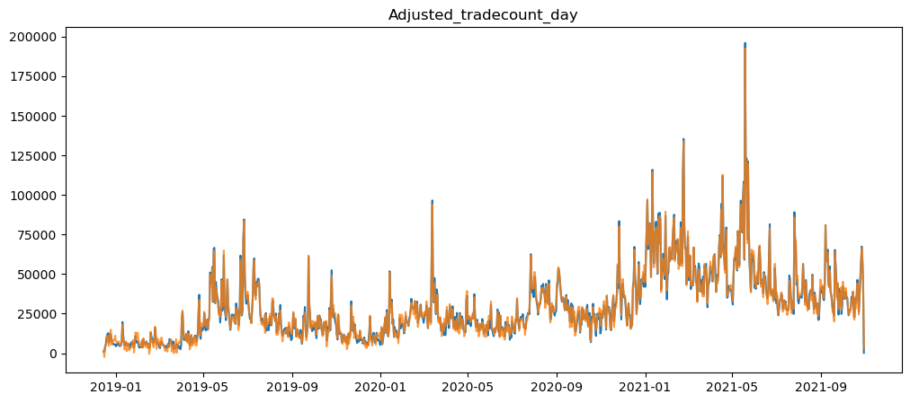
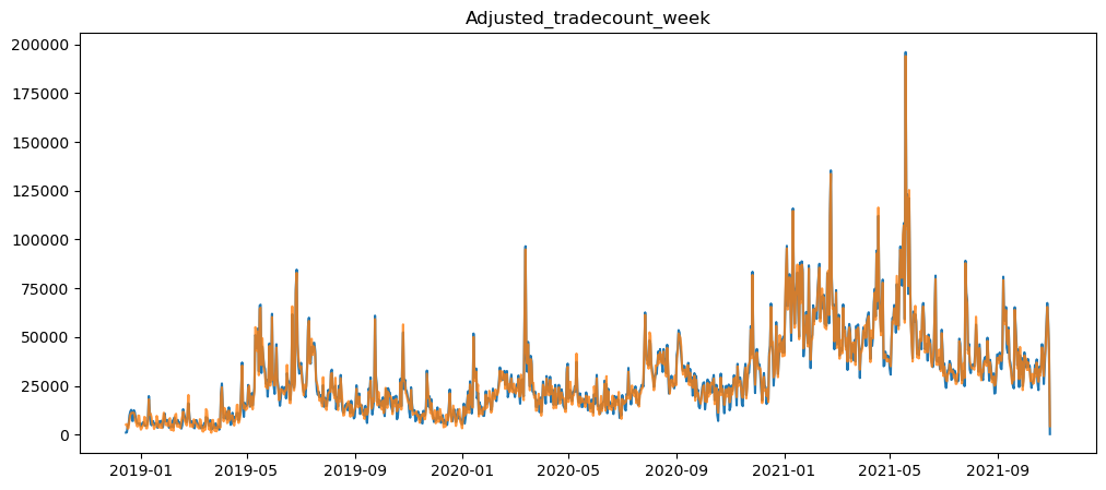

As shown above, only when using the month timeframe, where we can see that the graph moved only a little, and the seasonality of the graph was not removed.
Looking for Seasonality using FFT
We will try to use FFT to identify the seasonality in some of the dataset.
pd.Series(np.fft.fft(ticketSalesData)).plot()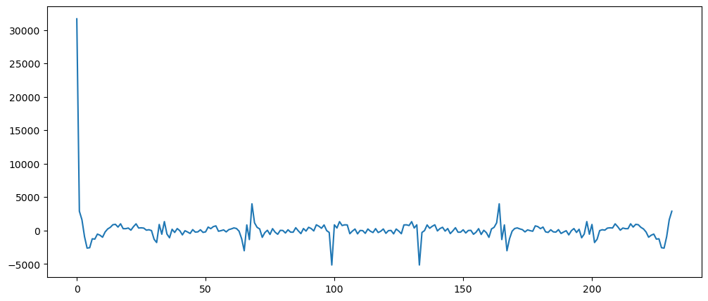
pd.Series(np.abs(np.fft.fft(ticketSalesData))).plot()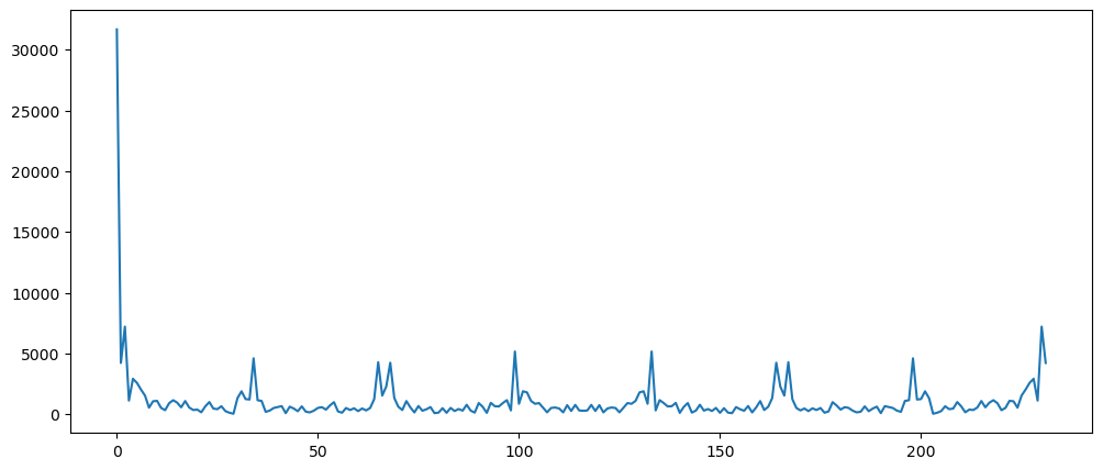
pd.Series(np.abs(np.fft.fft(ticketSalesData)[10:len(ticketSalesData)])).plot()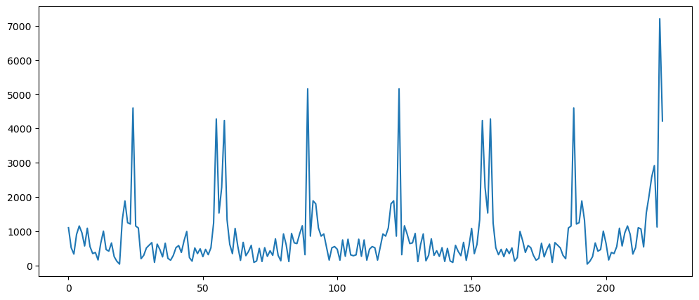
Clearly there are seasonality in this dataset
Gold
pd.Series(np.abs(np.fft.fft(goldData['Close'])[10:len(ticketSalesData)])).plot()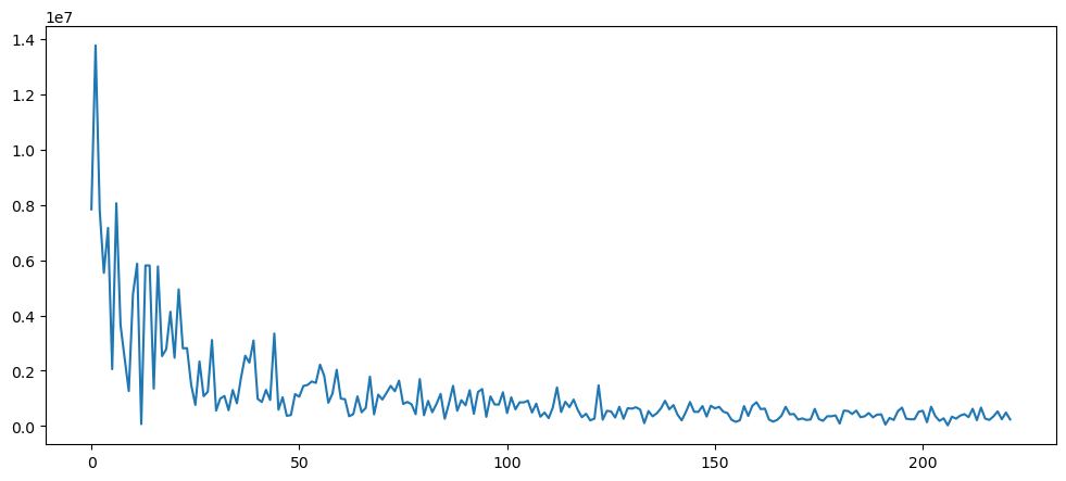
pd.Series(np.abs(np.fft.fft(goldData['Close'])[10:len(ticketSalesData)//3])).plot()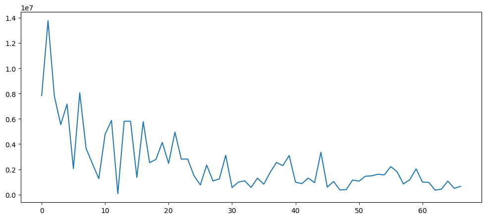
For gold, there seem to be no seasonality in the dataset.
Machine Learning Questions
pd.Series(np.abs(np.fft.fft(mlStackoverflow_data['machine-learning'])[0:len(ticketSalesData)])).plot()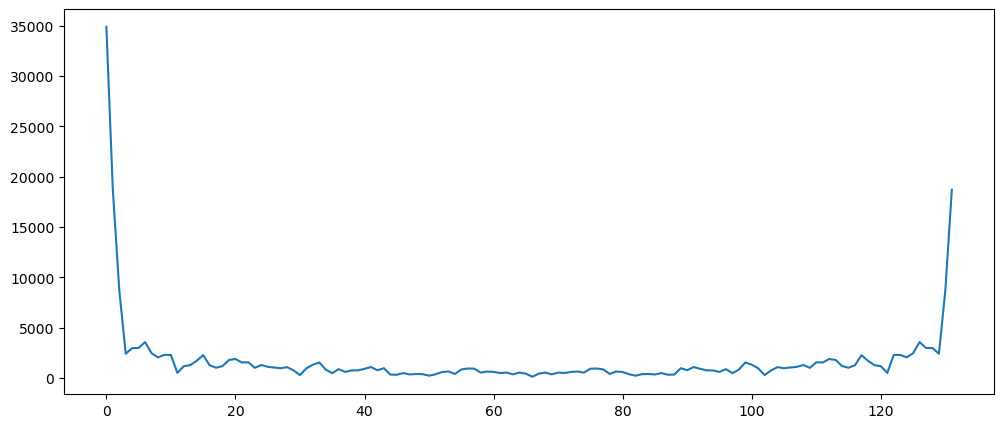
pd.Series(np.abs(np.fft.fft(mlStackoverflow_data['machine-learning'])[100:])).plot()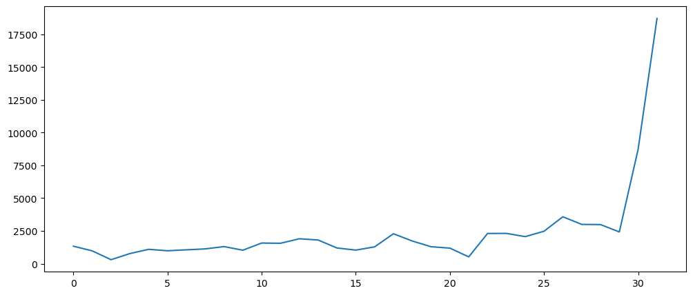
Honestly cannot tell if the final stretch of the values is considered to indicating that this dataset is a seasonal component
USDCUSDT Tradecount
usdcusdt_data['tradecount']0 277
1 43366
2 58314
3 67437
4 56204
...
1046 9876
1047 5308
1048 4360
1049 1185
1050 1054
Name: tradecount, Length: 1051, dtype: int64pd.Series(np.abs(np.fft.fft(usdcusdt_data['tradecount']))).plot()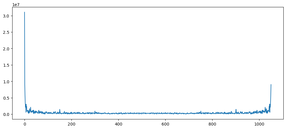
Clearly this is not a seasonal dataset.
Forecasting
Naive Forecasting
Taking the previous period as a prediction. Therefore, we only need to shift the column by one, as we have done for the differencing. Some example shown at the bottom.
def naiveForecasting(series):
temp = pd.DataFrame(series.rename('observed'))
temp.insert(1, 'predicted', temp['observed'].shift())
return tempmlTopicNaiveForecast = naiveForecasting(mlStackoverflow_data['machine-learning'])
mlTopicNaiveForecast.plot()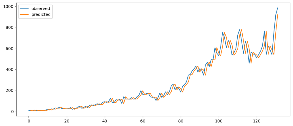
ticketSoldNaiveForecast = naiveForecasting(ticketSales_data['tickets_sold'])
ticketSoldNaiveForecast.plot()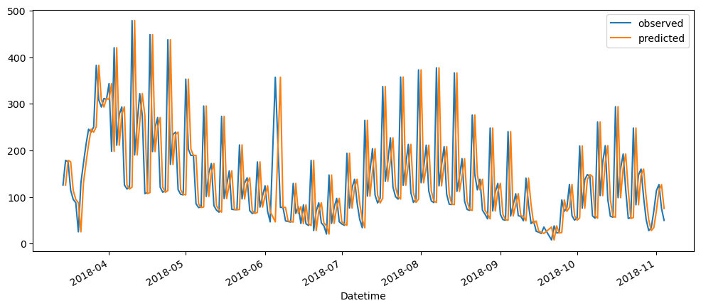
goldPriceNaiveForecast = naiveForecasting(gold_data['Close'])
goldPriceNaiveForecast.plot()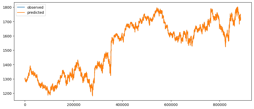
Seasonal Forecasting
Define a season and then we predict that next season with the previous season's value. It is similar to naive forecasting above, but with more time gap in between
def seasonalForecasting(series, season):
temp = pd.DataFrame(series.rename('observed'))
temp.insert(1, 'predicted', temp['observed'].shift(season))
return tempBecause each data point represents a month, our season could be quarter, half yearly or yearly.
mlTopicSeasonalYearlyForecast = seasonalForecasting(mlStackoverflow_data['machine-learning'], 12)
mlTopicSeasonalYearlyForecast.plot()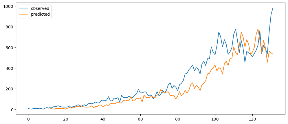
mlTopicSeasonalQuarterlyForecast = seasonalForecasting(mlStackoverflow_data['machine-learning'], 3)
mlTopicSeasonalQuarterlyForecast.plot()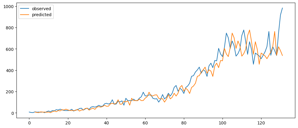
ticketSoldWeeklyForecast = seasonalForecasting(ticketSales_data['tickets_sold'], 7)
ticketSoldWeeklyForecast.plot()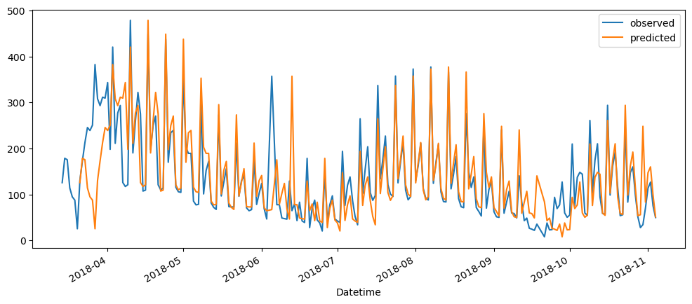
ticketSoldMonthlyForecast = seasonalForecasting(ticketSales_data['tickets_sold'], 30)
ticketSoldMonthlyForecast.plot()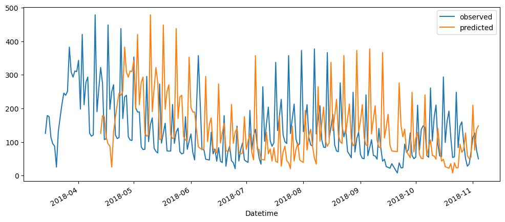
goldPriceDailyForecast = seasonalForecasting(gold_data['Close'], 1440)
goldPriceDailyForecast.plot()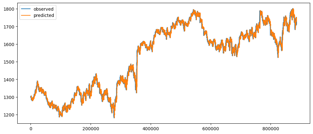
goldPriceWeeklyForecast = seasonalForecasting(gold_data['Close'], 10080)
goldPriceWeeklyForecast.plot()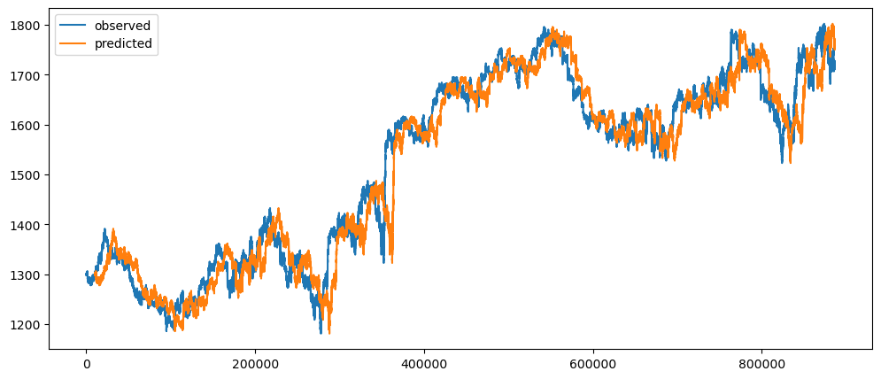
Average Forecasting
Using the average of the previous n of observation to predict.
def averageForecasting(series, n):
temp = pd.DataFrame(series.rename('observed'))
temp.insert(1, 'predicted',
1/n * (temp['observed'].cumsum().shift() - temp['observed'].cumsum().shift(n+1)))
return temp
def averageForecastPlot(series, list):
for n in list:
temp = averageForecasting(series,n)
plt.plot(temp['predicted'], label = 'n = ' + str(n))
plt.plot(temp['observed'], label='observed', linewidth=2, alpha=0.3, linestyle='dashed')
plt.legend()
plt.show()averageForecastPlot(mlStackoverflow_data['machine-learning'],[2,6,12,24])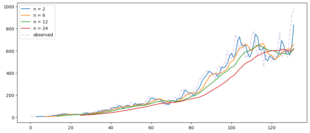
averageForecastPlot(ticketSales_data['tickets_sold'],[2,7,21,60])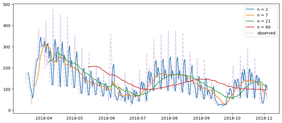
averageForecastPlot(gold_data['Close'],[1440,10080,43200])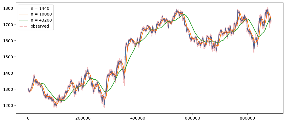
Based on the result shown, this method seem to be acting as a smoothing method rather than predictor, especially when it is with a longer time period.
Average Differences Forecasting
Now we will explore using average of the difference between timeframe, and use it as a way to predict
def differenceAverage(series, p):
temp = pd.DataFrame(series.rename('observed'))
difference = temp['observed'] - temp['observed'].shift()
prediction_of_differences = (1/p) * (difference.cumsum().shift(1) - difference.cumsum().shift(p+1))
temp['predicted']= prediction_of_differences.shift(1) + temp['observed'].shift(1)
return temp
def differenceAveragePlot(series, list):
plt.plot(series, label='observed', linewidth=2, alpha=0.5, linestyle='dashed')
for n in list:
plt.plot(differenceAverage(series, n)['predicted'], label='predicted, n = ' + str(n))
plt.legend()
plt.show()differenceAveragePlot(mlStackoverflow_data['machine-learning'], [2,6,12,24])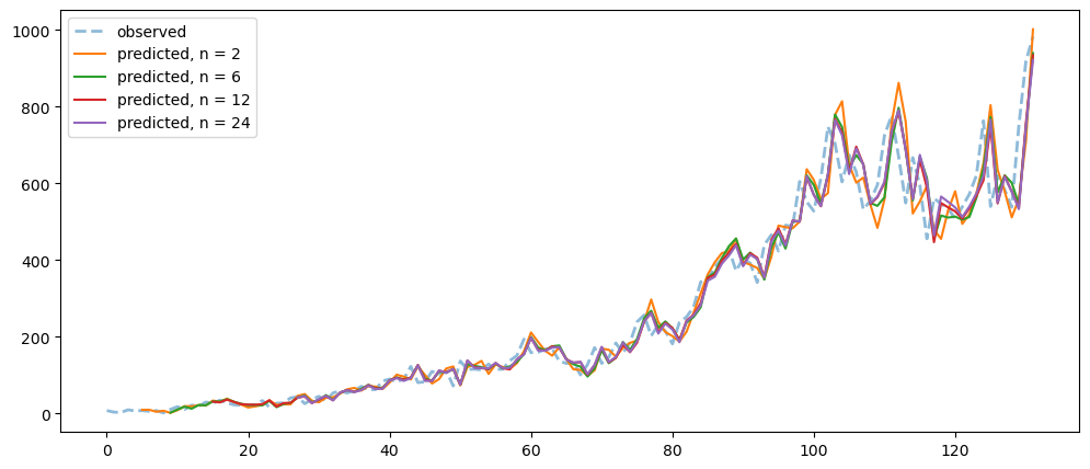
differenceAveragePlot(ticketSales_data['tickets_sold'], [2,6,12,24])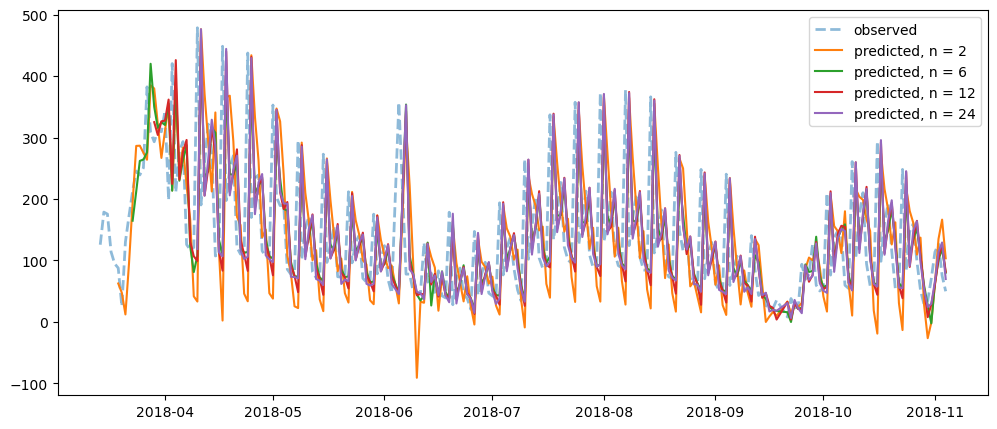
differenceAveragePlot(gold_data['Close'][:100000], [1440,10080,43200])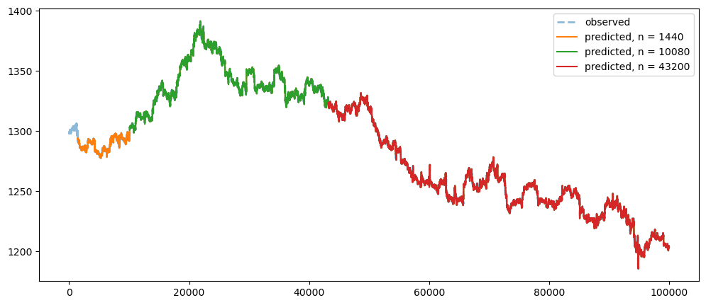
Naive Differences Forecasting
Make list the difference between the current period and previous period. Then, to predict the next value of the next period, take the difference from the current period and the previous period, and use it to predict the next value.
def naiveDifferenceForecasting(series):
temp = pd.DataFrame(series.rename('observed'))
differences = temp['observed'] - temp['observed'].shift()
predictionsOfDifferences = differences.shift()
temp['predicted'] = predictionsOfDifferences + temp['observed'].shift(1)
return tempnaiveDifferenceForecasting(mlStackoverflow_data['machine-learning']).plot()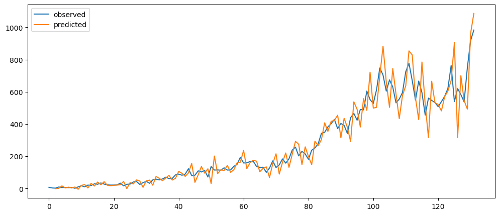
naiveForecasting(ticketSales_data['tickets_sold']).plot()
naiveDifferenceForecasting(gold_data['Close'])[:300].plot()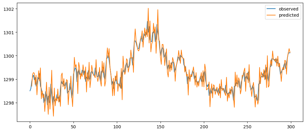
Ironic, that using a naive method, of use the previous change of value, to make a prediction, seem to be actually good. While based on the three dataset used, the prediction for the machine learning questions and gold prices, the prediction while it seems that it over-predicts the value, it does seem to at least predict the major movement same as the observed. But that might also be because it seems to be the case visually.
Evaluating the forecasts
Will now implement the ways we can use to evaluate the forecasts. We will be implementing MSE, RMSE and MAE, which are typically used for regression predictions.
Define Functions and Setting Table of Results
def mse(df):
temp = df['observed'] - df['predicted']
temp = temp**2
temp = temp.dropna()
return temp.sum() / temp.count()
def rmse(df):
return (mse(df))**(1/2)
def mae(df):
temp = abs(df['observed'] - df['predicted'])
temp = temp.dropna()
return temp.sum() / temp.count()
def evaluateErrors(df):
return [mse(df), rmse(df), mae(df)]tableOfResults = pd.DataFrame(columns = ['Data', 'Algorithm', 'MSE', 'RMSE', 'MAE'])
tableOfResults
# Function to fill the Table of Results
def appendingTOR(dataframe, dataset, algorithm, list):
dataframe.loc[len(dataframe)+1] = {'Data': dataset,'Algorithm': algorithm, 'MSE':list[0],'RMSE':list[1], 'MAE':list[2]}Naive Forecasting
# Re-setup some of the dataset above
sp500Data = sp500_data[['Datetime', 'Close']]
sp500Data = sp500Data.set_index('Datetime')
ftseData = ftse_data[['Datetime', 'Close']]
ftseData = ftseData.set_index('Datetime')
goldData = gold_data[['Datetime', 'Close']]
goldData = goldData.set_index('Datetime')
temp = usdcusdt_data[['date', 'close', 'tradecount']]
temp = temp.set_index(pd.to_datetime(temp['date']))
usdcusdtDataTradeCount = temp[['tradecount']]
usdcusdtDataClose = temp[['close']]
# Create Naive Forcast Predictions
sp500DataNaiveForecast = naiveForecasting(sp500Data['Close'])
ftseDataNaiveForecast = naiveForecasting(ftseData['Close'])
goldDataNaiveForecast = naiveForecasting(goldData['Close'])
usdcusdtDataCloseNaiveForecast = naiveForecasting(usdcusdtDataClose['close'])
usdcusdtTradeCountNaiveForecast = naiveForecasting(usdcusdtDataTradeCount['tradecount'])
pythonNaiveForecast = naiveForecasting(mlStackoverflow_data['python'])
# Appending to Result Table
naiveForecastingString = 'Naive Forecasting'
appendingTOR(tableOfResults, 'SP500', naiveForecastingString, evaluateErrors(sp500DataNaiveForecast))
appendingTOR(tableOfResults, 'FTSE', naiveForecastingString, evaluateErrors(ftseDataNaiveForecast))
appendingTOR(tableOfResults, 'Gold', naiveForecastingString, evaluateErrors(goldDataNaiveForecast))
appendingTOR(tableOfResults, 'USDCUSDT Close Price', naiveForecastingString, evaluateErrors(usdcusdtDataCloseNaiveForecast))
appendingTOR(tableOfResults, 'USDCUSDT Tradecount', naiveForecastingString, evaluateErrors(usdcusdtTradeCountNaiveForecast))
appendingTOR(tableOfResults, 'Python Questions', naiveForecastingString, evaluateErrors(pythonNaiveForecast))
appendingTOR(tableOfResults, 'Machine Learning Questions', naiveForecastingString, evaluateErrors(mlTopicNaiveForecast))
appendingTOR(tableOfResults, 'Ticket Sales', naiveForecastingString, evaluateErrors(ticketSoldNaiveForecast))
tableOfResults| Unnamed: 0 | Data | Algorithm | MSE | RMSE | MAE |
|---|---|---|---|---|---|
| 1 | SP500 | Naive Forecasting | 0.315878 | 0.56203 | 0.325863 |
| 2 | FTSE | Naive Forecasting | 5.69646 | 2.38673 | 1.29783 |
| 3 | Gold | Naive Forecasting | 0.237289 | 0.487123 | 0.31245 |
| 4 | USDCUSDT Close Price | Naive Forecasting | 4.01536e-06 | 0.002004 | 0.001034 |
| 5 | USDCUSDT Tradecount | Naive Forecasting | 1.56376e+08 | 12505 | 7519.96 |
| 6 | Python Questions | Naive Forecasting | 1.00863e+06 | 1004.31 | 680.298 |
| 7 | Machine Learning Questions | Naive Forecasting | 3053.46 | 55.2581 | 35.4885 |
| 8 | Ticket Sales | Naive Forecasting | 12476 | 111.696 | 74.8537 |
Seasonal Forecasting
# Create Seasonal Forecasting Predictions
sp500SeasonalForecast60 = seasonalForecasting(sp500Data['Close'], 60)
sp500SeasonalForecast1440 = seasonalForecasting(sp500Data['Close'], 1440)
ftseSeasonalForecast60 = seasonalForecasting(ftseData['Close'], 60)
ftseSeasonalForecast1440 = seasonalForecasting(ftseData['Close'], 1440)
goldSeasonalForecast60 = seasonalForecasting(goldData['Close'], 60)
goldSeasonalForecast1440 = seasonalForecasting(goldData['Close'], 1440)
usdcusdtCloseSeasonalForecast = seasonalForecasting(usdcusdtDataClose['close'], 7)
usdcusdtTCSeasonalForecast = seasonalForecasting(usdcusdtDataTradeCount['tradecount'], 7)
pythonSeasonalForecast = seasonalForecasting(mlStackoverflow_data['python'], 12)
# Appending to Result Table
seasonalForecastingString = 'Seasonal Forecasting'
appendingTOR(tableOfResults, 'SP500', seasonalForecastingString + ' - 60', evaluateErrors(sp500SeasonalForecast60))
appendingTOR(tableOfResults, 'SP500', seasonalForecastingString + ' - 1440', evaluateErrors(sp500SeasonalForecast1440))
appendingTOR(tableOfResults, 'FTSE', seasonalForecastingString + ' - 60', evaluateErrors(ftseSeasonalForecast60) )
appendingTOR(tableOfResults, 'FTSE', seasonalForecastingString + ' - 1440', evaluateErrors(ftseSeasonalForecast1440))
appendingTOR(tableOfResults, 'Gold', seasonalForecastingString + ' - 60', evaluateErrors(goldSeasonalForecast60))
appendingTOR(tableOfResults, 'Gold', seasonalForecastingString + ' - 1440', evaluateErrors(goldSeasonalForecast1440))
appendingTOR(tableOfResults, 'USDCUSDT Close Price', seasonalForecastingString, evaluateErrors(usdcusdtCloseSeasonalForecast))
appendingTOR(tableOfResults, 'USDCUSDT Tradecount', seasonalForecastingString, evaluateErrors(usdcusdtTCSeasonalForecast))
appendingTOR(tableOfResults, 'Python Questions', seasonalForecastingString, evaluateErrors(pythonSeasonalForecast))
appendingTOR(tableOfResults, 'Machine Learning Questions', seasonalForecastingString, evaluateErrors(mlTopicSeasonalYearlyForecast))
appendingTOR(tableOfResults, 'Ticket Sales', seasonalForecastingString, evaluateErrors(ticketSoldWeeklyForecast))
tableOfResults| Unnamed: 0 | Data | Algorithm | MSE | RMSE | MAE |
|---|---|---|---|---|---|
| 1 | SP500 | Naive Forecasting | 0.315878 | 0.56203 | 0.325863 |
| 2 | FTSE | Naive Forecasting | 5.69646 | 2.38673 | 1.29783 |
| 3 | Gold | Naive Forecasting | 0.237289 | 0.487123 | 0.31245 |
| 4 | USDCUSDT Close Price | Naive Forecasting | 4.01536e-06 | 0.002004 | 0.001034 |
| 5 | USDCUSDT Tradecount | Naive Forecasting | 1.56376e+08 | 12505 | 7519.96 |
| 6 | Python Questions | Naive Forecasting | 1.00863e+06 | 1004.31 | 680.298 |
| 7 | Machine Learning Questions | Naive Forecasting | 3053.46 | 55.2581 | 35.4885 |
| 8 | Ticket Sales | Naive Forecasting | 12476 | 111.696 | 74.8537 |
| 9 | SP500 | Seasonal Forecasting - 60 | 24.0706 | 4.90618 | 3.19858 |
| 10 | SP500 | Seasonal Forecasting - 1440 | 578.648 | 24.0551 | 18.6964 |
| 11 | FTSE | Seasonal Forecasting - 60 | 358.944 | 18.9458 | 12.5549 |
| 12 | FTSE | Seasonal Forecasting - 1440 | 9305.27 | 96.4639 | 71.5358 |
| 13 | Gold | Seasonal Forecasting - 60 | 11.0817 | 3.32892 | 2.08104 |
| 14 | Gold | Seasonal Forecasting - 1440 | 297.39 | 17.245 | 12.2358 |
| 15 | USDCUSDT Close Price | Seasonal Forecasting | 1.41478e-05 | 0.003761 | 0.00176 |
| 16 | USDCUSDT Tradecount | Seasonal Forecasting | 2.76653e+08 | 16632.9 | 10558.5 |
| 17 | Python Questions | Seasonal Forecasting | 4.97505e+06 | 2230.48 | 1924.32 |
| 18 | Machine Learning Questions | Seasonal Forecasting | 14325.5 | 119.689 | 84.975 |
| 19 | Ticket Sales | Seasonal Forecasting | 3922.4 | 62.6291 | 37.0187 |
Average Forecasting
# Create Average Forecasting Predictions
sp500AverageForecast60 = averageForecasting(sp500Data['Close'], 60)
sp500AverageForecast1440 = averageForecasting(sp500Data['Close'], 1440)
ftseAverageForecast60 = averageForecasting(ftseData['Close'], 60)
ftseAverageForecast1440 = averageForecasting(ftseData['Close'], 1440)
goldAverageForecast60 = averageForecasting(goldData['Close'], 60)
goldAverageForecast1440 = averageForecasting(goldData['Close'], 1440)
usdcusdtCloseAverageForecast = averageForecasting(usdcusdtDataClose['close'], 7)
usdcusdtTCAverageForecast = averageForecasting(usdcusdtDataTradeCount['tradecount'], 7)
pythonAverageForecast = averageForecasting(mlStackoverflow_data['python'], 12)
mlTopicAverageForecast = averageForecasting(mlStackoverflow_data['machine-learning'], 12)
ticketSalesAverageForecast = averageForecasting(ticketSales_data['tickets_sold'], 7)
# Appending to Result Table
averageForcastingString = 'Average Forecasting'
appendingTOR(tableOfResults, 'SP500', averageForcastingString + ' - 60', evaluateErrors(sp500AverageForecast60))
appendingTOR(tableOfResults, 'SP500', averageForcastingString + ' - 1440', evaluateErrors(sp500AverageForecast1440))
appendingTOR(tableOfResults, 'FTSE', averageForcastingString + ' - 60', evaluateErrors(ftseAverageForecast60))
appendingTOR(tableOfResults, 'FTSE', averageForcastingString + ' - 1440', evaluateErrors(ftseAverageForecast1440))
appendingTOR(tableOfResults, 'Gold', averageForcastingString + ' - 60', evaluateErrors(goldAverageForecast60))
appendingTOR(tableOfResults, 'Gold', averageForcastingString + ' - 1440', evaluateErrors(goldAverageForecast1440))
appendingTOR(tableOfResults, 'USDCUSDT Close Price', averageForcastingString, evaluateErrors(usdcusdtCloseAverageForecast))
appendingTOR(tableOfResults, 'USDCUSDT Tradecount', averageForcastingString, evaluateErrors(usdcusdtTCAverageForecast))
appendingTOR(tableOfResults, 'Python Questions', averageForcastingString, evaluateErrors(pythonAverageForecast))
appendingTOR(tableOfResults, 'Machine Learning Questions', averageForcastingString, evaluateErrors(mlTopicAverageForecast))
appendingTOR(tableOfResults, 'Ticket Sales', averageForcastingString, evaluateErrors(ticketSalesAverageForecast))
tableOfResults| Unnamed: 0 | Data | Algorithm | MSE | RMSE | MAE |
|---|---|---|---|---|---|
| 1 | SP500 | Naive Forecasting | 0.315878 | 0.56203 | 0.325863 |
| 2 | FTSE | Naive Forecasting | 5.69646 | 2.38673 | 1.29783 |
| 3 | Gold | Naive Forecasting | 0.237289 | 0.487123 | 0.31245 |
| 4 | USDCUSDT Close Price | Naive Forecasting | 4.01536e-06 | 0.002004 | 0.001034 |
| 5 | USDCUSDT Tradecount | Naive Forecasting | 1.56376e+08 | 12505 | 7519.96 |
| 6 | Python Questions | Naive Forecasting | 1.00863e+06 | 1004.31 | 680.298 |
| 7 | Machine Learning Questions | Naive Forecasting | 3053.46 | 55.2581 | 35.4885 |
| 8 | Ticket Sales | Naive Forecasting | 12476 | 111.696 | 74.8537 |
| 9 | SP500 | Seasonal Forecasting - 60 | 24.0706 | 4.90618 | 3.19858 |
| 10 | SP500 | Seasonal Forecasting - 1440 | 578.648 | 24.0551 | 18.6964 |
| 11 | FTSE | Seasonal Forecasting - 60 | 358.944 | 18.9458 | 12.5549 |
| 12 | FTSE | Seasonal Forecasting - 1440 | 9305.27 | 96.4639 | 71.5358 |
| 13 | Gold | Seasonal Forecasting - 60 | 11.0817 | 3.32892 | 2.08104 |
| 14 | Gold | Seasonal Forecasting - 1440 | 297.39 | 17.245 | 12.2358 |
| 15 | USDCUSDT Close Price | Seasonal Forecasting | 1.41478e-05 | 0.003761 | 0.00176 |
| 16 | USDCUSDT Tradecount | Seasonal Forecasting | 2.76653e+08 | 16632.9 | 10558.5 |
| 17 | Python Questions | Seasonal Forecasting | 4.97505e+06 | 2230.48 | 1924.32 |
| 18 | Machine Learning Questions | Seasonal Forecasting | 14325.5 | 119.689 | 84.975 |
| 19 | Ticket Sales | Seasonal Forecasting | 3922.4 | 62.6291 | 37.0187 |
| 20 | SP500 | Average Forecasting - 60 | 8.21104 | 2.86549 | 1.84062 |
| 21 | SP500 | Average Forecasting - 1440 | 195.085 | 13.9673 | 10.6287 |
| 22 | FTSE | Average Forecasting - 60 | 122.369 | 11.0621 | 7.24807 |
| 23 | FTSE | Average Forecasting - 1440 | 3105.82 | 55.7299 | 40.9431 |
| 24 | Gold | Average Forecasting - 60 | 3.79681 | 1.94854 | 1.22559 |
| 25 | Gold | Average Forecasting - 1440 | 96.5074 | 9.82382 | 6.8452 |
| 26 | USDCUSDT Close Price | Average Forecasting | 6.51406e-06 | 0.002552 | 0.001187 |
| 27 | USDCUSDT Tradecount | Average Forecasting | 1.44419e+08 | 12017.5 | 7727.27 |
| 28 | Python Questions | Average Forecasting | 2.18019e+06 | 1476.55 | 1175.32 |
| 29 | Machine Learning Questions | Average Forecasting | 7140.3 | 84.5003 | 55.785 |
| 30 | Ticket Sales | Average Forecasting | 6061.2 | 77.8537 | 59.7301 |
Average Differences
# Create Average Differences Prediction
sp500AverageDifferenceForecast60 = differenceAverage(sp500Data['Close'], 60)
sp500AverageDifferenceForecast1440 = differenceAverage(sp500Data['Close'], 1440)
ftseAverageDifferenceForecast60 = differenceAverage(ftseData['Close'], 60)
ftseAverageDifferenceForecast1440 = differenceAverage(ftseData['Close'], 1440)
goldAverageDifferenceForecast60 = differenceAverage(goldData['Close'], 60)
goldAverageDifferenceForecast1440 = differenceAverage(goldData['Close'], 1440)
usdcusdtCloseAverageDifferenceForecast = differenceAverage(usdcusdtDataClose['close'], 7)
usdcusdtTCAverageDifferenceForecast = differenceAverage(usdcusdtDataTradeCount['tradecount'], 7)
pythonAverageDifferenceForecast = differenceAverage(mlStackoverflow_data['python'], 12)
mlTopicAverageDifferenceForecast = differenceAverage(mlStackoverflow_data['machine-learning'], 12)
ticketSalesAverageDifferenceForecast = differenceAverage(ticketSales_data['tickets_sold'], 7)
# Appending to Result Table
averageDifferenceForecastingString = 'Average Difference Forecasting'
appendingTOR(tableOfResults, 'SP500', averageDifferenceForecastingString + ' - 60', evaluateErrors(sp500AverageDifferenceForecast60))
appendingTOR(tableOfResults, 'SP500', averageDifferenceForecastingString + ' - 1440', evaluateErrors(sp500AverageDifferenceForecast1440))
appendingTOR(tableOfResults, 'FTSE', averageDifferenceForecastingString + ' - 60', evaluateErrors(ftseAverageDifferenceForecast60))
appendingTOR(tableOfResults, 'FTSE', averageDifferenceForecastingString + ' - 1440', evaluateErrors(ftseAverageDifferenceForecast1440))
appendingTOR(tableOfResults, 'Gold', averageDifferenceForecastingString + ' - 60', evaluateErrors(goldAverageDifferenceForecast60))
appendingTOR(tableOfResults, 'Gold', averageDifferenceForecastingString + ' - 1440', evaluateErrors(goldAverageDifferenceForecast1440))
appendingTOR(tableOfResults, 'USDCUSDT Close Price', averageDifferenceForecastingString, evaluateErrors(usdcusdtCloseAverageDifferenceForecast))
appendingTOR(tableOfResults, 'USDCUSDT Tradecount', averageDifferenceForecastingString, evaluateErrors(usdcusdtTCAverageDifferenceForecast))
appendingTOR(tableOfResults, 'Python Questions', averageDifferenceForecastingString, evaluateErrors(pythonAverageDifferenceForecast))
appendingTOR(tableOfResults, 'Machine Learning Questions', averageDifferenceForecastingString, evaluateErrors(mlTopicAverageDifferenceForecast))
appendingTOR(tableOfResults, 'Ticket Sales', averageDifferenceForecastingString, evaluateErrors(ticketSalesAverageDifferenceForecast))
tableOfResults| Unnamed: 0 | Data | Algorithm | MSE | RMSE | MAE |
|---|---|---|---|---|---|
| 1 | SP500 | Naive Forecasting | 0.315878 | 0.56203 | 0.325863 |
| 2 | FTSE | Naive Forecasting | 5.69646 | 2.38673 | 1.29783 |
| 3 | Gold | Naive Forecasting | 0.237289 | 0.487123 | 0.31245 |
| 4 | USDCUSDT Close Price | Naive Forecasting | 4.01536e-06 | 0.002004 | 0.001034 |
| 5 | USDCUSDT Tradecount | Naive Forecasting | 1.56376e+08 | 12505 | 7519.96 |
| 6 | Python Questions | Naive Forecasting | 1.00863e+06 | 1004.31 | 680.298 |
| 7 | Machine Learning Questions | Naive Forecasting | 3053.46 | 55.2581 | 35.4885 |
| 8 | Ticket Sales | Naive Forecasting | 12476 | 111.696 | 74.8537 |
| 9 | SP500 | Seasonal Forecasting - 60 | 24.0706 | 4.90618 | 3.19858 |
| 10 | SP500 | Seasonal Forecasting - 1440 | 578.648 | 24.0551 | 18.6964 |
| 11 | FTSE | Seasonal Forecasting - 60 | 358.944 | 18.9458 | 12.5549 |
| 12 | FTSE | Seasonal Forecasting - 1440 | 9305.27 | 96.4639 | 71.5358 |
| 13 | Gold | Seasonal Forecasting - 60 | 11.0817 | 3.32892 | 2.08104 |
| 14 | Gold | Seasonal Forecasting - 1440 | 297.39 | 17.245 | 12.2358 |
| 15 | USDCUSDT Close Price | Seasonal Forecasting | 1.41478e-05 | 0.003761 | 0.00176 |
| 16 | USDCUSDT Tradecount | Seasonal Forecasting | 2.76653e+08 | 16632.9 | 10558.5 |
| 17 | Python Questions | Seasonal Forecasting | 4.97505e+06 | 2230.48 | 1924.32 |
| 18 | Machine Learning Questions | Seasonal Forecasting | 14325.5 | 119.689 | 84.975 |
| 19 | Ticket Sales | Seasonal Forecasting | 3922.4 | 62.6291 | 37.0187 |
| 20 | SP500 | Average Forecasting - 60 | 8.21104 | 2.86549 | 1.84062 |
| 21 | SP500 | Average Forecasting - 1440 | 195.085 | 13.9673 | 10.6287 |
| 22 | FTSE | Average Forecasting - 60 | 122.369 | 11.0621 | 7.24807 |
| 23 | FTSE | Average Forecasting - 1440 | 3105.82 | 55.7299 | 40.9431 |
| 24 | Gold | Average Forecasting - 60 | 3.79681 | 1.94854 | 1.22559 |
| 25 | Gold | Average Forecasting - 1440 | 96.5074 | 9.82382 | 6.8452 |
| 26 | USDCUSDT Close Price | Average Forecasting | 6.51406e-06 | 0.002552 | 0.001187 |
| 27 | USDCUSDT Tradecount | Average Forecasting | 1.44419e+08 | 12017.5 | 7727.27 |
| 28 | Python Questions | Average Forecasting | 2.18019e+06 | 1476.55 | 1175.32 |
| 29 | Machine Learning Questions | Average Forecasting | 7140.3 | 84.5003 | 55.785 |
| 30 | Ticket Sales | Average Forecasting | 6061.2 | 77.8537 | 59.7301 |
| 31 | SP500 | Average Difference Forecasting - 60 | 0.322452 | 0.567849 | 0.332982 |
| 32 | SP500 | Average Difference Forecasting - 1440 | 0.316412 | 0.562505 | 0.326336 |
| 33 | FTSE | Average Difference Forecasting - 60 | 5.79875 | 2.40806 | 1.32178 |
| 34 | FTSE | Average Difference Forecasting - 1440 | 5.70723 | 2.38898 | 1.30033 |
| 35 | Gold | Average Difference Forecasting - 60 | 0.240423 | 0.49033 | 0.315994 |
| 36 | Gold | Average Difference Forecasting - 1440 | 0.237595 | 0.487437 | 0.313009 |
| 37 | USDCUSDT Close Price | Average Difference Forecasting | 4.53094e-06 | 0.002129 | 0.001103 |
| 38 | USDCUSDT Tradecount | Average Difference Forecasting | 1.64095e+08 | 12810 | 7724.69 |
| 39 | Python Questions | Average Difference Forecasting | 1.1445e+06 | 1069.81 | 751.801 |
| 40 | Machine Learning Questions | Average Difference Forecasting | 3399.79 | 58.3077 | 38.5563 |
| 41 | Ticket Sales | Average Difference Forecasting | 12936.3 | 113.738 | 76.6102 |
Naive Difference
# Create Naive Difference Prediction
sp500NaiveDifferenceForecast = naiveDifferenceForecasting(sp500Data['Close'])
ftseNaiveDifferenceForecast = naiveDifferenceForecasting(ftseData['Close'])
goldNaiveDifferenceForecast = naiveDifferenceForecasting(goldData['Close'])
usdcusdtCloseNaiveDifferenceForecast = naiveDifferenceForecasting(usdcusdtDataClose['close'])
usdcusdtTCNaiveDifferenceForecast = naiveDifferenceForecasting(usdcusdtDataTradeCount['tradecount'])
pythonNaiveDifferenceForecast = naiveDifferenceForecasting(mlStackoverflow_data['python'])
mlTopicNaiveDifferenceForecast = naiveDifferenceForecasting(mlStackoverflow_data['machine-learning'])
ticketSalesNaiveDifferenceForecast = naiveDifferenceForecasting(ticketSales_data['tickets_sold'])
# Appending to Result Table
naiveDifferenceForecastingString = 'Naive Difference Forecasting'
appendingTOR(tableOfResults, 'SP500', naiveDifferenceForecastingString, evaluateErrors(sp500NaiveDifferenceForecast))
appendingTOR(tableOfResults, 'FTSE', naiveDifferenceForecastingString, evaluateErrors(ftseNaiveDifferenceForecast))
appendingTOR(tableOfResults, 'Gold', naiveDifferenceForecastingString, evaluateErrors(goldNaiveDifferenceForecast))
appendingTOR(tableOfResults, 'USDCUSDT Close Price', naiveDifferenceForecastingString, evaluateErrors(usdcusdtCloseNaiveDifferenceForecast))
appendingTOR(tableOfResults, 'USDCUSDT Tradecount', naiveDifferenceForecastingString, evaluateErrors(usdcusdtTCNaiveDifferenceForecast))
appendingTOR(tableOfResults, 'Python Questions', naiveDifferenceForecastingString, evaluateErrors(pythonNaiveDifferenceForecast))
appendingTOR(tableOfResults, 'Machine Learning Questions', naiveDifferenceForecastingString, evaluateErrors(mlTopicNaiveDifferenceForecast))
appendingTOR(tableOfResults, 'Ticket Sales', naiveDifferenceForecastingString, evaluateErrors(ticketSalesNaiveDifferenceForecast))
tableOfResults| Unnamed: 0 | Data | Algorithm | MSE | RMSE | MAE |
|---|---|---|---|---|---|
| 1 | SP500 | Naive Forecasting | 0.315878 | 0.56203 | 0.325863 |
| 2 | FTSE | Naive Forecasting | 5.69646 | 2.38673 | 1.29783 |
| 3 | Gold | Naive Forecasting | 0.237289 | 0.487123 | 0.31245 |
| 4 | USDCUSDT Close Price | Naive Forecasting | 4.01536e-06 | 0.002004 | 0.001034 |
| 5 | USDCUSDT Tradecount | Naive Forecasting | 1.56376e+08 | 12505 | 7519.96 |
| 6 | Python Questions | Naive Forecasting | 1.00863e+06 | 1004.31 | 680.298 |
| 7 | Machine Learning Questions | Naive Forecasting | 3053.46 | 55.2581 | 35.4885 |
| 8 | Ticket Sales | Naive Forecasting | 12476 | 111.696 | 74.8537 |
| 9 | SP500 | Seasonal Forecasting - 60 | 24.0706 | 4.90618 | 3.19858 |
| 10 | SP500 | Seasonal Forecasting - 1440 | 578.648 | 24.0551 | 18.6964 |
| 11 | FTSE | Seasonal Forecasting - 60 | 358.944 | 18.9458 | 12.5549 |
| 12 | FTSE | Seasonal Forecasting - 1440 | 9305.27 | 96.4639 | 71.5358 |
| 13 | Gold | Seasonal Forecasting - 60 | 11.0817 | 3.32892 | 2.08104 |
| 14 | Gold | Seasonal Forecasting - 1440 | 297.39 | 17.245 | 12.2358 |
| 15 | USDCUSDT Close Price | Seasonal Forecasting | 1.41478e-05 | 0.003761 | 0.00176 |
| 16 | USDCUSDT Tradecount | Seasonal Forecasting | 2.76653e+08 | 16632.9 | 10558.5 |
| 17 | Python Questions | Seasonal Forecasting | 4.97505e+06 | 2230.48 | 1924.32 |
| 18 | Machine Learning Questions | Seasonal Forecasting | 14325.5 | 119.689 | 84.975 |
| 19 | Ticket Sales | Seasonal Forecasting | 3922.4 | 62.6291 | 37.0187 |
| 20 | SP500 | Average Forecasting - 60 | 8.21104 | 2.86549 | 1.84062 |
| 21 | SP500 | Average Forecasting - 1440 | 195.085 | 13.9673 | 10.6287 |
| 22 | FTSE | Average Forecasting - 60 | 122.369 | 11.0621 | 7.24807 |
| 23 | FTSE | Average Forecasting - 1440 | 3105.82 | 55.7299 | 40.9431 |
| 24 | Gold | Average Forecasting - 60 | 3.79681 | 1.94854 | 1.22559 |
| 25 | Gold | Average Forecasting - 1440 | 96.5074 | 9.82382 | 6.8452 |
| 26 | USDCUSDT Close Price | Average Forecasting | 6.51406e-06 | 0.002552 | 0.001187 |
| 27 | USDCUSDT Tradecount | Average Forecasting | 1.44419e+08 | 12017.5 | 7727.27 |
| 28 | Python Questions | Average Forecasting | 2.18019e+06 | 1476.55 | 1175.32 |
| 29 | Machine Learning Questions | Average Forecasting | 7140.3 | 84.5003 | 55.785 |
| 30 | Ticket Sales | Average Forecasting | 6061.2 | 77.8537 | 59.7301 |
| 31 | SP500 | Average Difference Forecasting - 60 | 0.322452 | 0.567849 | 0.332982 |
| 32 | SP500 | Average Difference Forecasting - 1440 | 0.316412 | 0.562505 | 0.326336 |
| 33 | FTSE | Average Difference Forecasting - 60 | 5.79875 | 2.40806 | 1.32178 |
| 34 | FTSE | Average Difference Forecasting - 1440 | 5.70723 | 2.38898 | 1.30033 |
| 35 | Gold | Average Difference Forecasting - 60 | 0.240423 | 0.49033 | 0.315994 |
| 36 | Gold | Average Difference Forecasting - 1440 | 0.237595 | 0.487437 | 0.313009 |
| 37 | USDCUSDT Close Price | Average Difference Forecasting | 4.53094e-06 | 0.002129 | 0.001103 |
| 38 | USDCUSDT Tradecount | Average Difference Forecasting | 1.64095e+08 | 12810 | 7724.69 |
| 39 | Python Questions | Average Difference Forecasting | 1.1445e+06 | 1069.81 | 751.801 |
| 40 | Machine Learning Questions | Average Difference Forecasting | 3399.79 | 58.3077 | 38.5563 |
| 41 | Ticket Sales | Average Difference Forecasting | 12936.3 | 113.738 | 76.6102 |
| 42 | SP500 | Naive Difference Forecasting | 0.553753 | 0.744146 | 0.456603 |
| 43 | FTSE | Naive Difference Forecasting | 10.796 | 3.28573 | 1.81081 |
| 44 | Gold | Naive Difference Forecasting | 0.521205 | 0.721946 | 0.480641 |
| 45 | USDCUSDT Close Price | Naive Difference Forecasting | 9.13676e-06 | 0.003023 | 0.001659 |
| 46 | USDCUSDT Tradecount | Naive Difference Forecasting | 4.15266e+08 | 20378.1 | 12089.8 |
| 47 | Python Questions | Naive Difference Forecasting | 2.34416e+06 | 1531.07 | 1117.71 |
| 48 | Machine Learning Questions | Naive Difference Forecasting | 6678.13 | 81.7198 | 51.9462 |
| 49 | Ticket Sales | Naive Difference Forecasting | 37594.4 | 193.893 | 136.398 |
Analysis
Because the evaluation metrics does not produce a standardize output, we cannot use the MSE, RMSE, and MAE value directly without context. It needs to be compared within the same dataset used. For example, the evaluations on USDCUSDT dataset are the lowest, but that does not mean that average difference algorithm on usdcusdt is better than naive difference forecasting on Ticket Sales. So let's pick S&P500, Python Questions and Ticket Sales, to compare first and see what observations can we find.
display(tableOfResults[tableOfResults['Data'] == 'SP500'].sort_values('MSE'),
tableOfResults[tableOfResults['Data'] == 'Python Questions'].sort_values('MSE'),
tableOfResults[tableOfResults['Data'] == 'Ticket Sales'].sort_values('MSE'),
)| Unnamed: 0 | Data | Algorithm | MSE | RMSE | MAE |
|---|---|---|---|---|---|
| 1 | SP500 | Naive Forecasting | 0.315878 | 0.56203 | 0.325863 |
| 32 | SP500 | Average Difference Forecasting - 1440 | 0.316412 | 0.562505 | 0.326336 |
| 31 | SP500 | Average Difference Forecasting - 60 | 0.322453 | 0.567849 | 0.332982 |
| 42 | SP500 | Naive Difference Forecasting | 0.553753 | 0.744146 | 0.456603 |
| 20 | SP500 | Average Forecasting - 60 | 8.21104 | 2.86549 | 1.84062 |
| 9 | SP500 | Seasonal Forecasting - 60 | 24.0706 | 4.90618 | 3.19858 |
| 21 | SP500 | Average Forecasting - 1440 | 195.085 | 13.9673 | 10.6287 |
| 10 | SP500 | Seasonal Forecasting - 1440 | 578.648 | 24.0551 | 18.6964 |
| Unnamed: 0 | Data | Algorithm | MSE | RMSE | MAE |
|---|---|---|---|---|---|
| 6 | Python Questions | Naive Forecasting | 1.00863e+06 | 1004.31 | 680.298 |
| 39 | Python Questions | Average Difference Forecasting | 1.1445e+06 | 1069.81 | 751.801 |
| 28 | Python Questions | Average Forecasting | 2.18019e+06 | 1476.55 | 1175.32 |
| 47 | Python Questions | Naive Difference Forecasting | 2.34416e+06 | 1531.07 | 1117.71 |
| 17 | Python Questions | Seasonal Forecasting | 4.97505e+06 | 2230.48 | 1924.32 |
| Unnamed: 0 | Data | Algorithm | MSE | RMSE | MAE |
|---|---|---|---|---|---|
| 19 | Ticket Sales | Seasonal Forecasting | 3922.4 | 62.6291 | 37.0187 |
| 30 | Ticket Sales | Average Forecasting | 6061.2 | 77.8537 | 59.7301 |
| 8 | Ticket Sales | Naive Forecasting | 12476 | 111.696 | 74.8537 |
| 41 | Ticket Sales | Average Difference Forecasting | 12936.3 | 113.738 | 76.6102 |
| 49 | Ticket Sales | Naive Difference Forecasting | 37594.4 | 193.893 | 136.398 |
We can see that all of there evaluation value are very different in terms of size and magnitude. Then, currently we can see that naive forecasting performing the best. Let's list all the best algorithm for the given dataset.
for dataset in tableOfResults['Data'].unique():
display(tableOfResults[tableOfResults['Data'] == dataset].sort_values('MSE').head(2))| Unnamed: 0 | Data | Algorithm | MSE | RMSE | MAE |
|---|---|---|---|---|---|
| 1 | SP500 | Naive Forecasting | 0.315878 | 0.56203 | 0.325863 |
| 32 | SP500 | Average Difference Forecasting - 1440 | 0.316412 | 0.562505 | 0.326336 |
| Unnamed: 0 | Data | Algorithm | MSE | RMSE | MAE |
|---|---|---|---|---|---|
| 2 | FTSE | Naive Forecasting | 5.69646 | 2.38673 | 1.29783 |
| 34 | FTSE | Average Difference Forecasting - 1440 | 5.70723 | 2.38898 | 1.30033 |
| Unnamed: 0 | Data | Algorithm | MSE | RMSE | MAE |
|---|---|---|---|---|---|
| 3 | Gold | Naive Forecasting | 0.237289 | 0.487123 | 0.31245 |
| 36 | Gold | Average Difference Forecasting - 1440 | 0.237595 | 0.487437 | 0.313009 |
| Unnamed: 0 | Data | Algorithm | MSE | RMSE | MAE |
|---|---|---|---|---|---|
| 4 | USDCUSDT Close Price | Naive Forecasting | 4e-06 | 0.002004 | 0.001034 |
| 37 | USDCUSDT Close Price | Average Difference Forecasting | 5e-06 | 0.002129 | 0.001103 |
| Unnamed: 0 | Data | Algorithm | MSE | RMSE | MAE |
|---|---|---|---|---|---|
| 27 | USDCUSDT Tradecount | Average Forecasting | 1.44419e+08 | 12017.5 | 7727.27 |
| 5 | USDCUSDT Tradecount | Naive Forecasting | 1.56376e+08 | 12505 | 7519.96 |
| Unnamed: 0 | Data | Algorithm | MSE | RMSE | MAE |
|---|---|---|---|---|---|
| 6 | Python Questions | Naive Forecasting | 1.00863e+06 | 1004.31 | 680.298 |
| 39 | Python Questions | Average Difference Forecasting | 1.1445e+06 | 1069.81 | 751.801 |
| Unnamed: 0 | Data | Algorithm | MSE | RMSE | MAE |
|---|---|---|---|---|---|
| 7 | Machine Learning Questions | Naive Forecasting | 3053.46 | 55.2581 | 35.4885 |
| 40 | Machine Learning Questions | Average Difference Forecasting | 3399.79 | 58.3077 | 38.5563 |
| Unnamed: 0 | Data | Algorithm | MSE | RMSE | MAE |
|---|---|---|---|---|---|
| 19 | Ticket Sales | Seasonal Forecasting | 3922.4 | 62.6291 | 37.0187 |
| 30 | Ticket Sales | Average Forecasting | 6061.2 | 77.8537 | 59.7301 |
We can observe that Naive Forecasting seem to be the best choice at the moment, and the Average Difference in second. Only TicketSales and USDCUSDT Tradecount do not have both of the algorithm. This could be because the ticket sales and usdcusdt datasets, have more prominent repeatable pattern that other forecasting methods work better, while because the rest of the dataset are more random in nature.
Additionally, something to take note is that Naive Forecasting and Average Differences are currently the best algorithm only in the context of technical evaluation of MSE, RMSE and MAE. Because if we were to set trading/investment rules and different way to evaluate performance, the result might be different.
Autoregression Prediction
Before we can use autoregression prediction, first we will need to make the datasets stationary, as well as using autocorrelation and partial autocorrelation.
Choosing Dataset
We have a lot of datasets that we can use. We will use ticket sales (because it consists of more obvious seasonal changes), machine learning questions from stackoverflow (for its multiplicativeness), SP500 and Gold dataset as they are real world financial data. But because the SP500 and Gold data are very large, we will only use 3 months of data.
We will need need to also split the dataset into training and testing sets. We will use 70% as training and 30% training.
Autocorrelation and Partial Autocorrelation
# Importing plot_acf
from statsmodels.graphics.tsaplots import plot_acf, plot_pacfGold Data
Making it stationary
stationaryGoldData = goldData
stationaryGoldData['observed'] = goldData['Close'] - goldData['Close'].shift()
stationaryGoldData = stationaryGoldData.dropna().drop('Close', axis=1)
stationaryGoldData = stationaryGoldData[stationaryGoldData.index.dayofweek != 5]
stationaryGoldData = stationaryGoldData[:108000]
kpss_test(stationaryGoldData)
print()
adftest(stationaryGoldData)
stationaryGoldData.plot()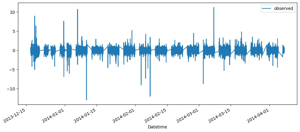
Setting the training and testing set
stationaryGoldDataLength = len(stationaryGoldData)
traniningStationaryGoldDataLength = int(len(stationaryGoldData) * 0.7)
testingStationaryGoldDataLength = stationaryGoldDataLength - traniningStationaryGoldDataLength
print(stationaryGoldDataLength, traniningStationaryGoldDataLength, testingStationaryGoldDataLength)108000 75600 32400ACF
plot_acf(stationaryGoldData[:traniningStationaryGoldDataLength],lags=60)
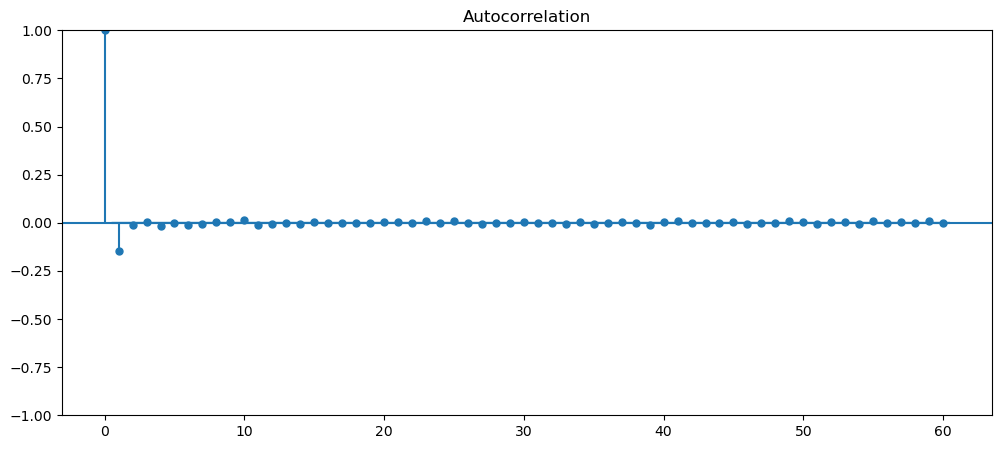
PACF
plot_pacf(stationaryGoldData[:traniningStationaryGoldDataLength], lags = 60)
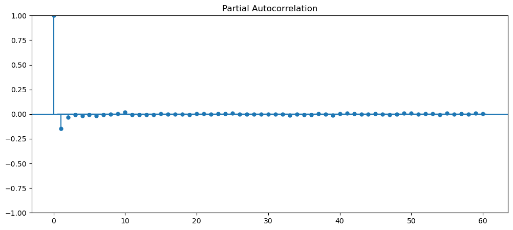
S&P500
Making it stationary
stationarySP500Data = sp500Data
stationarySP500Data['observed'] = sp500Data['Close'] - sp500Data['Close'].shift()
stationarySP500Data = stationarySP500Data.dropna().drop('Close', axis=1)
stationarySP500Data = stationarySP500Data[stationarySP500Data.index.dayofweek != 5].sort_index()
stationarySP500Data = stationarySP500Data[:36000]
kpss_test(stationarySP500Data)
print()
adftest(stationarySP500Data)
stationarySP500Data.plot()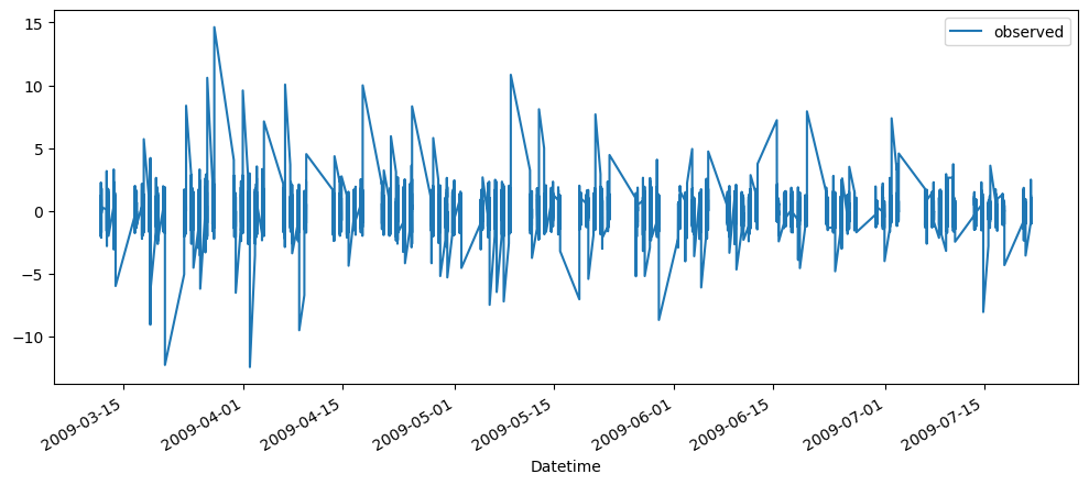
Setting the training and testing set
stationarySP500DataLength = len(stationarySP500Data)
trainingStationarySP500Data = int(0.7 * stationarySP500DataLength)
testingStationarySP500Data = stationarySP500DataLength - trainingStationarySP500Data
print(stationarySP500DataLength, trainingStationarySP500Data, testingStationarySP500Data)36000 25200 10800ACF
plot_acf(stationarySP500Data[:trainingStationarySP500Data], lags=60)
plt.xticks([x for x in range(0,61,2)])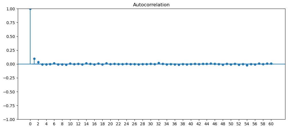
PACF
plot_pacf(stationarySP500Data[:trainingStationarySP500Data], lags=60)
plt.xticks([x for x in range(0,61,2)])
Machine Learning Questions
Because the dataset is multiplicative, we will need to log and get the difference of it.
Making it Stationary
stationaryMLQuestions = mlStackoverflow_data[['month','machine-learning']]
# Setting the month as index and also removing the month column.
stationaryMLQuestions = stationaryMLQuestions.set_index(
pd.to_datetime(stationaryMLQuestions['month'],format='%y-%b'
)).drop('month', axis=1)
stationaryMLQuestions = np.log(stationaryMLQuestions)
stationaryMLQuestions.plot()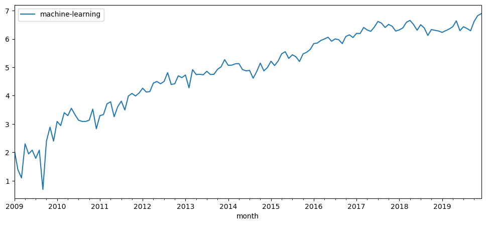
kpss_test(stationaryMLQuestions)
print()
adftest(stationaryMLQuestions)KPSS Stat: 1.873246798025978
p-value: 0.01
Number of lags: 6
Critial Values:
10% : 0.347
5% : 0.463
2.5% : 0.574
1% : 0.739
Result: The series is not stationary
AdfTest Stat: -2.668195595640323
p-value: 0.07970535704695508
Number of lags: 2
Number of observation: 129
Critial Values:
1% : -3.482087964046026
5% : -2.8842185101614626
10% : -2.578864381347275
The series is not stationarystationaryMLQuestions['observed'] = stationaryMLQuestions['machine-learning'] - stationaryMLQuestions['machine-learning'].shift()
stationaryMLQuestions = stationaryMLQuestions.dropna().drop('machine-learning', axis=1)
stationaryMLQuestions.plot()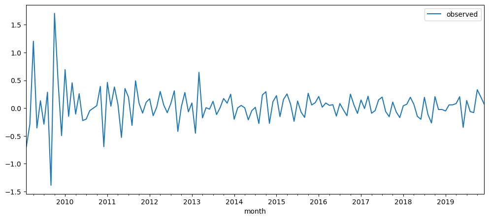
kpss_test(stationaryMLQuestions)
print()
adftest(stationaryMLQuestions)KPSS Stat: 0.28055757025438893
p-value: 0.1
Number of lags: 55
Critial Values:
10% : 0.347
5% : 0.463
2.5% : 0.574
1% : 0.739
Result: The series is stationary
AdfTest Stat:  -13.691197822513615
p-value:  1.342938733545792e-25
Number of lags: 1
Number of observation: 129
Critial Values:
   1% : -3.482087964046026
   5% : -2.8842185101614626
   10% : -2.578864381347275
The series is stationarySetting the training and testing set
stationaryMLQuestionsLength = len(stationaryMLQuestions)
trainingStationaryMLQuestions = int(stationaryMLQuestionsLength * 0.7)
testingStationaryMLQuestions = stationaryMLQuestionsLength - trainingStationaryMLQuestions

print(stationaryMLQuestionsLength, trainingStationaryMLQuestions, testingStationaryMLQuestions )
131 91 40ACF
plot_acf(stationaryMLQuestions[:trainingStationaryMLQuestions], lags=60)
plt.xticks([x for x in range(0,61,2)])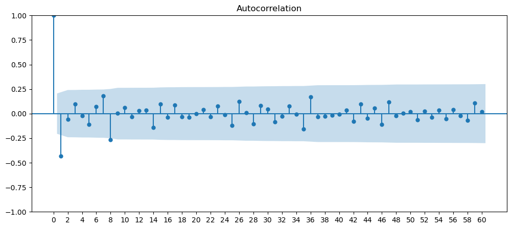
PACF
plot_pacf(stationaryMLQuestions[:trainingStationaryMLQuestions], lags=44)
plt.xticks([x for x in range(0,45,2)])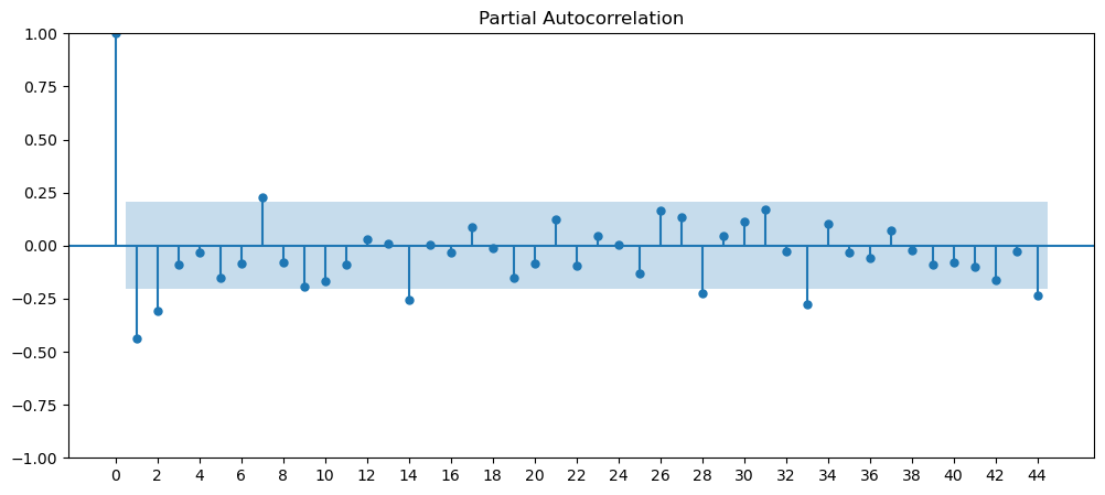
Cinema Tickets
Making it Stationary
stationaryTicketSales = ticketSales_data
stationaryTicketSales['observed'] = stationaryTicketSales['tickets_sold'] - stationaryTicketSales['tickets_sold'].shift()
stationaryTicketSales = stationaryTicketSales['observed'].dropna()

kpss_test(stationaryTicketSales)
print()
adftest(stationaryTicketSales)
KPSS Stat: 0.14388225215810577
p-value: 0.1
Number of lags: 62
Critial Values:
10% : 0.347
5% : 0.463
2.5% : 0.574
1% : 0.739
Result: The series is stationary
AdfTest Stat: -6.734609879307423
p-value: 3.2311867005854417e-09
Number of lags: 12
Number of observation: 218
Critial Values:
1% : -3.460707667106296
5% : -2.874891213486339
10% : -2.573885987711472
The series is stationarystationaryTicketSales.plot()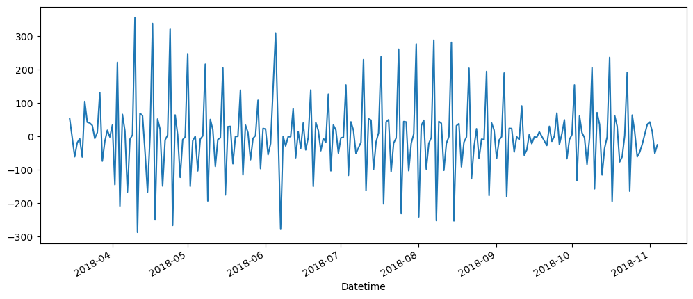
Setting the training set and testing set
stationaryTicketSalesLength = len(stationaryTicketSales)
trainingStationaryTicketSales = int(stationaryTicketSalesLength * 0.7)
testingStationaryTicketSales = stationaryTicketSalesLength - trainingStationaryTicketSales

print(stationaryTicketSalesLength, trainingStationaryTicketSales, testingStationaryTicketSales)
231 161 70ACF
plot_acf(stationaryTicketSales[:trainingStationaryTicketSales], lags=60)
plt.xticks([x for x in range(0,60,2)])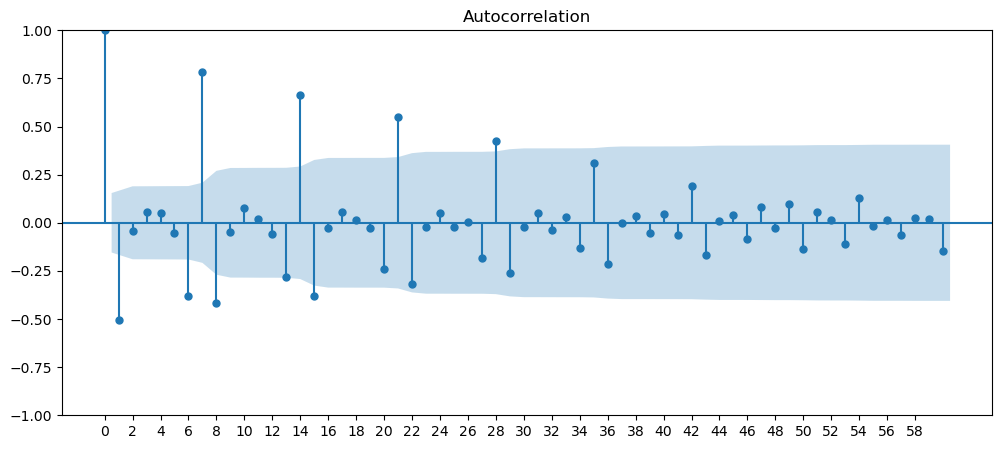
PACF
plot_pacf(stationaryTicketSales[:trainingStationaryTicketSales], lags=60)
plt.xticks([x for x in range(0,61,2)])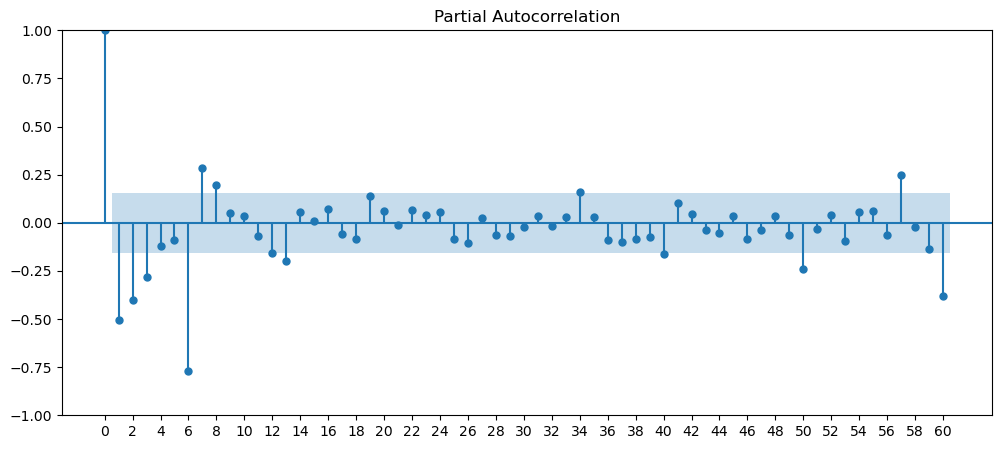
Prediction
We will be moving on with the prediction portion. We will be using the outputs from the PACF to determine the lags/period that we will be using for the autoregression.
Gold
from statsmodels.tsa.ar_model import AutoReggoldResults = AutoReg(stationaryGoldData[:traniningStationaryGoldDataLength], [1,2,3]).fit()
goldResults.summary()AutoReg Model Results
| Dep. Variable: | observed | No. Observations: | 75600 |
| Model: | AutoReg(3) | Log Likelihood | -30274.411 |
| Method: | Conditional MLE | S.D. of innovations | 0.361 |
| Date: | Mon, 08 Jul 2024 | AIC | 60558.822 |
| Time: | 15:38:54 | BIC | 60604.988 |
| Sample: | 3 | HQIC | 60573.011 |
| 75600 |
| coef | std err | z | P>|z| | [0.025 | 0.975] | |
|---|---|---|---|---|---|---|
| const | -0.0008 | 0.001 | -0.617 | 0.537 | -0.003 | 0.002 |
| observed.L1 | -0.1528 | 0.004 | -42.018 | 0.000 | -0.160 | -0.146 |
| observed.L2 | -0.0332 | 0.004 | -9.021 | 0.000 | -0.040 | -0.026 |
| observed.L3 | -0.0047 | 0.004 | -1.282 | 0.200 | -0.012 | 0.002 |
Roots
| Real | Imaginary | Modulus | Frequency | |
|---|---|---|---|---|
| AR.1 | -0.1166 | -5.5814j | 5.5827 | -0.2533 |
| AR.2 | -0.1166 | +5.5814j | 5.5827 | 0.2533 |
| AR.3 | -6.8805 | -0.0000j | 6.8805 | -0.5000 |
goldResults.paramsconst -0.000811
observed.L1 -0.152820
observed.L2 -0.033173
observed.L3 -0.004663
dtype: float64predictions = goldResults.predict(start=traniningStationaryGoldDataLength, end=stationaryGoldDataLength-1) + \
gold_data['Close'].shift()[traniningStationaryGoldDataLength:stationaryGoldDataLength]
stationaryGoldDataResults = pd.DataFrame(goldData.reset_index()['Close'][traniningStationaryGoldDataLength:stationaryGoldDataLength].rename('observed'))
stationaryGoldDataResults['predicted'] = predictions
stationaryGoldDataResults.plot()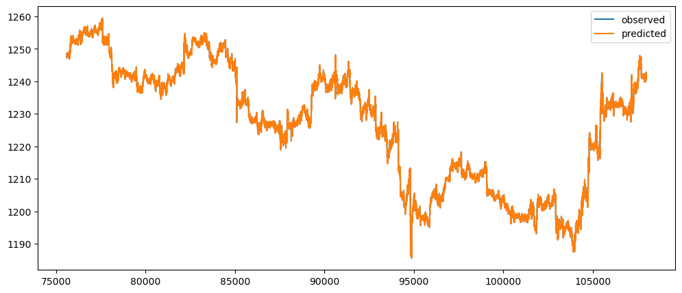
appendingTOR(tableOfResults, 'Gold', 'Autoregression', evaluateErrors(stationaryGoldDataResults))
tableOfResults| Unnamed: 0 | Data | Algorithm | MSE | RMSE | MAE |
|---|---|---|---|---|---|
| 1 | SP500 | Naive Forecasting | 0.315878 | 0.56203 | 0.325863 |
| 2 | FTSE | Naive Forecasting | 5.69646 | 2.38673 | 1.29783 |
| 3 | Gold | Naive Forecasting | 0.237289 | 0.487123 | 0.31245 |
| 4 | USDCUSDT Close Price | Naive Forecasting | 4.01536e-06 | 0.002004 | 0.001034 |
| 5 | USDCUSDT Tradecount | Naive Forecasting | 1.56376e+08 | 12505 | 7519.96 |
| 6 | Python Questions | Naive Forecasting | 1.00863e+06 | 1004.31 | 680.298 |
| 7 | Machine Learning Questions | Naive Forecasting | 3053.46 | 55.2581 | 35.4885 |
| 8 | Ticket Sales | Naive Forecasting | 12476 | 111.696 | 74.8537 |
| 9 | SP500 | Seasonal Forecasting - 60 | 24.0706 | 4.90618 | 3.19858 |
| 10 | SP500 | Seasonal Forecasting - 1440 | 578.648 | 24.0551 | 18.6964 |
| 11 | FTSE | Seasonal Forecasting - 60 | 358.944 | 18.9458 | 12.5549 |
| 12 | FTSE | Seasonal Forecasting - 1440 | 9305.27 | 96.4639 | 71.5358 |
| 13 | Gold | Seasonal Forecasting - 60 | 11.0817 | 3.32892 | 2.08104 |
| 14 | Gold | Seasonal Forecasting - 1440 | 297.39 | 17.245 | 12.2358 |
| 15 | USDCUSDT Close Price | Seasonal Forecasting | 1.41478e-05 | 0.003761 | 0.00176 |
| 16 | USDCUSDT Tradecount | Seasonal Forecasting | 2.76653e+08 | 16632.9 | 10558.5 |
| 17 | Python Questions | Seasonal Forecasting | 4.97505e+06 | 2230.48 | 1924.32 |
| 18 | Machine Learning Questions | Seasonal Forecasting | 14325.5 | 119.689 | 84.975 |
| 19 | Ticket Sales | Seasonal Forecasting | 3922.4 | 62.6291 | 37.0187 |
| 20 | SP500 | Average Forecasting - 60 | 8.21104 | 2.86549 | 1.84062 |
| 21 | SP500 | Average Forecasting - 1440 | 195.085 | 13.9673 | 10.6287 |
| 22 | FTSE | Average Forecasting - 60 | 122.369 | 11.0621 | 7.24807 |
| 23 | FTSE | Average Forecasting - 1440 | 3105.82 | 55.7299 | 40.9431 |
| 24 | Gold | Average Forecasting - 60 | 3.79681 | 1.94854 | 1.22559 |
| 25 | Gold | Average Forecasting - 1440 | 96.5074 | 9.82382 | 6.8452 |
| 26 | USDCUSDT Close Price | Average Forecasting | 6.51406e-06 | 0.002552 | 0.001187 |
| 27 | USDCUSDT Tradecount | Average Forecasting | 1.44419e+08 | 12017.5 | 7727.27 |
| 28 | Python Questions | Average Forecasting | 2.18019e+06 | 1476.55 | 1175.32 |
| 29 | Machine Learning Questions | Average Forecasting | 7140.3 | 84.5003 | 55.785 |
| 30 | Ticket Sales | Average Forecasting | 6061.2 | 77.8537 | 59.7301 |
| 31 | SP500 | Average Difference Forecasting - 60 | 0.322452 | 0.567849 | 0.332982 |
| 32 | SP500 | Average Difference Forecasting - 1440 | 0.316412 | 0.562505 | 0.326336 |
| 33 | FTSE | Average Difference Forecasting - 60 | 5.79875 | 2.40806 | 1.32178 |
| 34 | FTSE | Average Difference Forecasting - 1440 | 5.70723 | 2.38898 | 1.30033 |
| 35 | Gold | Average Difference Forecasting - 60 | 0.240423 | 0.49033 | 0.315994 |
| 36 | Gold | Average Difference Forecasting - 1440 | 0.237595 | 0.487437 | 0.313009 |
| 37 | USDCUSDT Close Price | Average Difference Forecasting | 4.53094e-06 | 0.002129 | 0.001103 |
| 38 | USDCUSDT Tradecount | Average Difference Forecasting | 1.64095e+08 | 12810 | 7724.69 |
| 39 | Python Questions | Average Difference Forecasting | 1.1445e+06 | 1069.81 | 751.801 |
| 40 | Machine Learning Questions | Average Difference Forecasting | 3399.79 | 58.3077 | 38.5563 |
| 41 | Ticket Sales | Average Difference Forecasting | 12936.3 | 113.738 | 76.6102 |
| 42 | SP500 | Naive Difference Forecasting | 0.553753 | 0.744146 | 0.456603 |
| 43 | FTSE | Naive Difference Forecasting | 10.796 | 3.28573 | 1.81081 |
| 44 | Gold | Naive Difference Forecasting | 0.521205 | 0.721946 | 0.480641 |
| 45 | USDCUSDT Close Price | Naive Difference Forecasting | 9.13676e-06 | 0.003023 | 0.001659 |
| 46 | USDCUSDT Tradecount | Naive Difference Forecasting | 4.15266e+08 | 20378.1 | 12089.8 |
| 47 | Python Questions | Naive Difference Forecasting | 2.34416e+06 | 1531.07 | 1117.71 |
| 48 | Machine Learning Questions | Naive Difference Forecasting | 6678.13 | 81.7198 | 51.9462 |
| 49 | Ticket Sales | Naive Difference Forecasting | 37594.4 | 193.893 | 136.398 |
| 50 | Gold | Autoregression | 0.167187 | 0.408885 | 0.270593 |
S&P500
sp500Results = AutoReg(stationarySP500Data[:trainingStationarySP500Data],[1,2,3]).fit()
sp500Results.summary()
AutoReg Model Results
| Dep. Variable: | observed | No. Observations: | 25200 |
| Model: | AutoReg(3) | Log Likelihood | -26406.1 |
| Method: | Conditional MLE | S.D. of innovations | 0.69 |
| Date: | Mon, 08 Jul 2024 | AIC | 52822.1 |
| Time: | 15:38:55 | BIC | 52862.8 |
| Sample: | 3 | HQIC | 52835.3 |
| 25200 |
| coef | std err | z | P>|z| | [0.025 | 0.975] | |
|---|---|---|---|---|---|---|
| const | -0.0081 | 0.004 | -1.865 | 0.062 | -0.017 | 0.000 |
| observed.L1 | 0.0963 | 0.006 | 15.284 | 0.000 | 0.084 | 0.109 |
| observed.L2 | 0.0258 | 0.006 | 4.074 | 0.000 | 0.013 | 0.038 |
| observed.L3 | -0.0102 | 0.006 | -1.612 | 0.107 | -0.023 | 0.002 |
Roots
| Real | Imaginary | Modulus | Frequency | |
|---|---|---|---|---|
| AR.1 | -4.4810 | -0.0000j | 4.4810 | -0.5000 |
| AR.2 | 3.5094 | -3.1074j | 4.6874 | -0.1153 |
| AR.3 | 3.5094 | +3.1074j | 4.6874 | 0.1153 |
sp500Data['Close'].shift()[trainingStationarySP500Data: stationarySP500DataLength]Datetime
2014-01-03 15:43:00 1837.18
2014-01-03 15:42:00 1837.49
2014-01-03 15:41:00 1837.61
2014-01-03 15:40:00 1837.14
2014-01-03 15:39:00 1836.72
...
2013-11-20 20:39:00 1780.69
2013-11-20 20:38:00 1779.84
2013-11-20 20:37:00 1779.54
2013-11-20 20:36:00 1779.17
2013-11-20 20:35:00 1778.87
Name: Close, Length: 10800, dtype: float64sp500Results.predict(start=trainingStationarySP500Data, end=stationarySP500DataLength-1)c:\Users\Edwin Teoh\anaconda3\lib\site-packages\statsmodels\tsa\base\tsa_model.py:834: ValueWarning: No supported index is available. Prediction results will be given with an integer index beginning at `start`.
return get_prediction_index(
c:\Users\Edwin Teoh\anaconda3\lib\site-packages\statsmodels\tsa\deterministic.py:302: UserWarning: Only PeriodIndexes, DatetimeIndexes with a frequency set, RangesIndexes, and Index with a unit increment support extending. The index is set will contain the position relative to the data length.
fcast_index = self._extend_index(index, steps, forecast_index)25200 0.005949
25201 -0.002961
25202 -0.009767
25203 -0.009188
25204 -0.009218
...
35995 -0.009133
35996 -0.009133
35997 -0.009133
35998 -0.009133
35999 -0.009133
Length: 10800, dtype: float64predictions = sp500Results.predict(start=trainingStationarySP500Data, end=stationarySP500DataLength-1) + \
sp500Data.reset_index()['Close'].shift()[trainingStationarySP500Data: stationarySP500DataLength]
stationarySP500DataResults = pd.DataFrame(
sp500Data.reset_index()['Close'][trainingStationarySP500Data:stationarySP500DataLength].rename('observed'))
stationarySP500DataResults['predicted'] = predictions
stationarySP500DataResults.plot()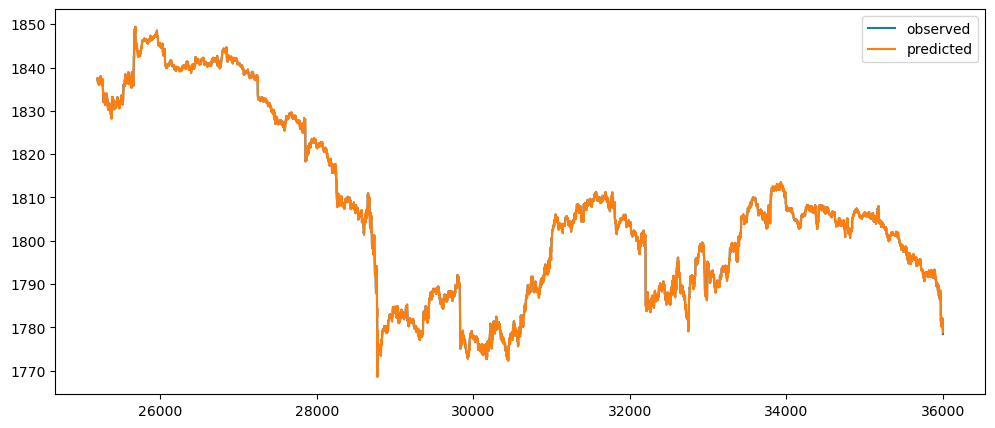
appendingTOR(tableOfResults, 'SP500', 'Autoregression', evaluateErrors(stationarySP500DataResults))
tableOfResults| Unnamed: 0 | Data | Algorithm | MSE | RMSE | MAE |
|---|---|---|---|---|---|
| 1 | SP500 | Naive Forecasting | 0.315878 | 0.56203 | 0.325863 |
| 2 | FTSE | Naive Forecasting | 5.69646 | 2.38673 | 1.29783 |
| 3 | Gold | Naive Forecasting | 0.237289 | 0.487123 | 0.31245 |
| 4 | USDCUSDT Close Price | Naive Forecasting | 4.01536e-06 | 0.002004 | 0.001034 |
| 5 | USDCUSDT Tradecount | Naive Forecasting | 1.56376e+08 | 12505 | 7519.96 |
| 6 | Python Questions | Naive Forecasting | 1.00863e+06 | 1004.31 | 680.298 |
| 7 | Machine Learning Questions | Naive Forecasting | 3053.46 | 55.2581 | 35.4885 |
| 8 | Ticket Sales | Naive Forecasting | 12476 | 111.696 | 74.8537 |
| 9 | SP500 | Seasonal Forecasting - 60 | 24.0706 | 4.90618 | 3.19858 |
| 10 | SP500 | Seasonal Forecasting - 1440 | 578.648 | 24.0551 | 18.6964 |
| 11 | FTSE | Seasonal Forecasting - 60 | 358.944 | 18.9458 | 12.5549 |
| 12 | FTSE | Seasonal Forecasting - 1440 | 9305.27 | 96.4639 | 71.5358 |
| 13 | Gold | Seasonal Forecasting - 60 | 11.0817 | 3.32892 | 2.08104 |
| 14 | Gold | Seasonal Forecasting - 1440 | 297.39 | 17.245 | 12.2358 |
| 15 | USDCUSDT Close Price | Seasonal Forecasting | 1.41478e-05 | 0.003761 | 0.00176 |
| 16 | USDCUSDT Tradecount | Seasonal Forecasting | 2.76653e+08 | 16632.9 | 10558.5 |
| 17 | Python Questions | Seasonal Forecasting | 4.97505e+06 | 2230.48 | 1924.32 |
| 18 | Machine Learning Questions | Seasonal Forecasting | 14325.5 | 119.689 | 84.975 |
| 19 | Ticket Sales | Seasonal Forecasting | 3922.4 | 62.6291 | 37.0187 |
| 20 | SP500 | Average Forecasting - 60 | 8.21104 | 2.86549 | 1.84062 |
| 21 | SP500 | Average Forecasting - 1440 | 195.085 | 13.9673 | 10.6287 |
| 22 | FTSE | Average Forecasting - 60 | 122.369 | 11.0621 | 7.24807 |
| 23 | FTSE | Average Forecasting - 1440 | 3105.82 | 55.7299 | 40.9431 |
| 24 | Gold | Average Forecasting - 60 | 3.79681 | 1.94854 | 1.22559 |
| 25 | Gold | Average Forecasting - 1440 | 96.5074 | 9.82382 | 6.8452 |
| 26 | USDCUSDT Close Price | Average Forecasting | 6.51406e-06 | 0.002552 | 0.001187 |
| 27 | USDCUSDT Tradecount | Average Forecasting | 1.44419e+08 | 12017.5 | 7727.27 |
| 28 | Python Questions | Average Forecasting | 2.18019e+06 | 1476.55 | 1175.32 |
| 29 | Machine Learning Questions | Average Forecasting | 7140.3 | 84.5003 | 55.785 |
| 30 | Ticket Sales | Average Forecasting | 6061.2 | 77.8537 | 59.7301 |
| 31 | SP500 | Average Difference Forecasting - 60 | 0.322452 | 0.567849 | 0.332982 |
| 32 | SP500 | Average Difference Forecasting - 1440 | 0.316412 | 0.562505 | 0.326336 |
| 33 | FTSE | Average Difference Forecasting - 60 | 5.79875 | 2.40806 | 1.32178 |
| 34 | FTSE | Average Difference Forecasting - 1440 | 5.70723 | 2.38898 | 1.30033 |
| 35 | Gold | Average Difference Forecasting - 60 | 0.240423 | 0.49033 | 0.315994 |
| 36 | Gold | Average Difference Forecasting - 1440 | 0.237595 | 0.487437 | 0.313009 |
| 37 | USDCUSDT Close Price | Average Difference Forecasting | 4.53094e-06 | 0.002129 | 0.001103 |
| 38 | USDCUSDT Tradecount | Average Difference Forecasting | 1.64095e+08 | 12810 | 7724.69 |
| 39 | Python Questions | Average Difference Forecasting | 1.1445e+06 | 1069.81 | 751.801 |
| 40 | Machine Learning Questions | Average Difference Forecasting | 3399.79 | 58.3077 | 38.5563 |
| 41 | Ticket Sales | Average Difference Forecasting | 12936.3 | 113.738 | 76.6102 |
| 42 | SP500 | Naive Difference Forecasting | 0.553753 | 0.744146 | 0.456603 |
| 43 | FTSE | Naive Difference Forecasting | 10.796 | 3.28573 | 1.81081 |
| 44 | Gold | Naive Difference Forecasting | 0.521205 | 0.721946 | 0.480641 |
| 45 | USDCUSDT Close Price | Naive Difference Forecasting | 9.13676e-06 | 0.003023 | 0.001659 |
| 46 | USDCUSDT Tradecount | Naive Difference Forecasting | 4.15266e+08 | 20378.1 | 12089.8 |
| 47 | Python Questions | Naive Difference Forecasting | 2.34416e+06 | 1531.07 | 1117.71 |
| 48 | Machine Learning Questions | Naive Difference Forecasting | 6678.13 | 81.7198 | 51.9462 |
| 49 | Ticket Sales | Naive Difference Forecasting | 37594.4 | 193.893 | 136.398 |
| 50 | Gold | Autoregression | 0.167187 | 0.408885 | 0.270593 |
| 51 | SP500 | Autoregression | 0.181846 | 0.426434 | 0.236095 |
Machine Learning Questions
mlQuestionsResults = AutoReg(stationaryMLQuestions[:trainingStationaryMLQuestions], [1, 2, 7, 14, 28, 31]).fit()
mlQuestionsResults.summary()
AutoReg Model Results
| Dep. Variable: | observed | No. Observations: | 91 |
| Model: | Restr. AutoReg(31) | Log Likelihood | 24.827 |
| Method: | Conditional MLE | S.D. of innovations | 0.16 |
| Date: | Mon, 08 Jul 2024 | AIC | -33.654 |
| Time: | 15:38:55 | BIC | -16.899 |
| Sample: | 09-01-2011 | HQIC | -27.1 |
| - 08-01-2016 |
| coef | std err | z | P>|z| | [0.025 | 0.975] | |
|---|---|---|---|---|---|---|
| const | 0.0658 | 0.023 | 2.894 | 0.004 | 0.021 | 0.110 |
| observed.L1 | -0.4974 | 0.116 | -4.289 | 0.000 | -0.725 | -0.270 |
| observed.L2 | -0.2309 | 0.124 | -1.862 | 0.063 | -0.474 | 0.012 |
| observed.L7 | 0.2036 | 0.099 | 2.049 | 0.040 | 0.009 | 0.398 |
| observed.L14 | -0.0429 | 0.089 | -0.483 | 0.629 | -0.217 | 0.131 |
| observed.L28 | -0.0634 | 0.055 | -1.158 | 0.247 | -0.171 | 0.044 |
| observed.L31 | -0.0349 | 0.050 | -0.695 | 0.487 | -0.133 | 0.064 |
Roots
| Real | Imaginary | Modulus | Frequency | |
|---|---|---|---|---|
| AR.1 | -0.8987 | -0.5721j | 1.0654 | -0.4098 |
| AR.2 | -0.8987 | +0.5721j | 1.0654 | 0.4098 |
| AR.3 | -1.0050 | -0.3868j | 1.0769 | -0.4415 |
| AR.4 | -1.0050 | +0.3868j | 1.0769 | 0.4415 |
| AR.5 | -1.1138 | -0.1904j | 1.1300 | -0.4731 |
| AR.6 | -1.1138 | +0.1904j | 1.1300 | 0.4731 |
| AR.7 | -1.2513 | -0.0000j | 1.2513 | -0.5000 |
| AR.8 | -0.7733 | -0.7617j | 1.0854 | -0.3762 |
| AR.9 | -0.7733 | +0.7617j | 1.0854 | 0.3762 |
| AR.10 | -0.5650 | -0.9155j | 1.0758 | -0.3380 |
| AR.11 | -0.5650 | +0.9155j | 1.0758 | 0.3380 |
| AR.12 | -0.3691 | -0.9883j | 1.0550 | -0.3069 |
| AR.13 | -0.3691 | +0.9883j | 1.0550 | 0.3069 |
| AR.14 | -0.1692 | -1.0598j | 1.0732 | -0.2752 |
| AR.15 | -0.1692 | +1.0598j | 1.0732 | 0.2752 |
| AR.16 | 0.0585 | -1.1078j | 1.1094 | -0.2416 |
| AR.17 | 0.0585 | +1.1078j | 1.1094 | 0.2416 |
| AR.18 | 1.0930 | -0.1180j | 1.0994 | -0.0171 |
| AR.19 | 1.0930 | +0.1180j | 1.0994 | 0.0171 |
| AR.20 | 1.0568 | -0.3488j | 1.1128 | -0.0507 |
| AR.21 | 1.0568 | +0.3488j | 1.1128 | 0.0507 |
| AR.22 | 0.9596 | -0.5937j | 1.1284 | -0.0882 |
| AR.23 | 0.9596 | +0.5937j | 1.1284 | 0.0882 |
| AR.24 | 0.8043 | -0.7902j | 1.1275 | -0.1236 |
| AR.25 | 0.8043 | +0.7902j | 1.1275 | 0.1236 |
| AR.26 | 0.3333 | -1.0889j | 1.1387 | -0.2027 |
| AR.27 | 0.3333 | +1.0889j | 1.1387 | 0.2027 |
| AR.28 | 0.6337 | -1.0033j | 1.1867 | -0.1603 |
| AR.29 | 0.6337 | +1.0033j | 1.1867 | 0.1603 |
| AR.30 | 0.5806 | -1.0452j | 1.1956 | -0.1693 |
| AR.31 | 0.5806 | +1.0452j | 1.1956 | 0.1693 |
loggedMLtopic0 2.079442
1 1.386294
2 1.098612
3 2.302585
4 1.945910
...
127 6.368187
128 6.287859
129 6.620073
130 6.822197
131 6.890609
Name: machine-learning, Length: 132, dtype: float64# Predictions from AR
predictions = mlQuestionsResults.predict(start = trainingStationaryMLQuestions, end = stationaryMLQuestionsLength-1).reset_index()
# Setting the index to number
predictions['index'] = [x for x in range(trainingStationaryMLQuestions,stationaryMLQuestionsLength)]
predictions = predictions.set_index('index')
# Adding the previous logged value
predictions = predictions[0] + loggedMLtopic.shift()
# Exponent it back
predictions = np.exp(predictions)
predictionsc:\Users\Edwin Teoh\anaconda3\lib\site-packages\statsmodels\tsa\deterministic.py:302: UserWarning: Only PeriodIndexes, DatetimeIndexes with a frequency set, RangesIndexes, and Index with a unit increment support extending. The index is set will contain the position relative to the data length.
fcast_index = self._extend_index(index, steps, forecast_index)0 NaN
1 NaN
2 NaN
3 NaN
4 NaN
...
127 642.365437
128 605.731054
129 561.555450
130 781.032565
131 NaN
Length: 132, dtype: float64stationaryMLQuestionsResults = pd.DataFrame(
mlStackoverflow_data['machine-learning'][trainingStationaryMLQuestions:stationaryMLQuestionsLength]
.rename('observed'))
stationaryMLQuestionsResults['predicted'] = predictions
stationaryMLQuestionsResults.plot()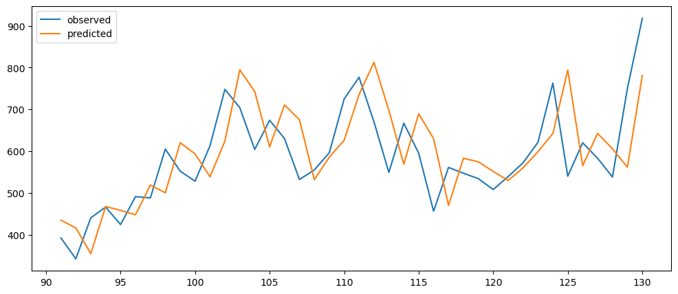
appendingTOR(tableOfResults, 'Machine Learning Questions', 'Autoregression', evaluateErrors(stationaryMLQuestionsResults))
tableOfResults| Unnamed: 0 | Data | Algorithm | MSE | RMSE | MAE |
|---|---|---|---|---|---|
| 1 | SP500 | Naive Forecasting | 0.315878 | 0.56203 | 0.325863 |
| 2 | FTSE | Naive Forecasting | 5.69646 | 2.38673 | 1.29783 |
| 3 | Gold | Naive Forecasting | 0.237289 | 0.487123 | 0.31245 |
| 4 | USDCUSDT Close Price | Naive Forecasting | 4.01536e-06 | 0.002004 | 0.001034 |
| 5 | USDCUSDT Tradecount | Naive Forecasting | 1.56376e+08 | 12505 | 7519.96 |
| 6 | Python Questions | Naive Forecasting | 1.00863e+06 | 1004.31 | 680.298 |
| 7 | Machine Learning Questions | Naive Forecasting | 3053.46 | 55.2581 | 35.4885 |
| 8 | Ticket Sales | Naive Forecasting | 12476 | 111.696 | 74.8537 |
| 9 | SP500 | Seasonal Forecasting - 60 | 24.0706 | 4.90618 | 3.19858 |
| 10 | SP500 | Seasonal Forecasting - 1440 | 578.648 | 24.0551 | 18.6964 |
| 11 | FTSE | Seasonal Forecasting - 60 | 358.944 | 18.9458 | 12.5549 |
| 12 | FTSE | Seasonal Forecasting - 1440 | 9305.27 | 96.4639 | 71.5358 |
| 13 | Gold | Seasonal Forecasting - 60 | 11.0817 | 3.32892 | 2.08104 |
| 14 | Gold | Seasonal Forecasting - 1440 | 297.39 | 17.245 | 12.2358 |
| 15 | USDCUSDT Close Price | Seasonal Forecasting | 1.41478e-05 | 0.003761 | 0.00176 |
| 16 | USDCUSDT Tradecount | Seasonal Forecasting | 2.76653e+08 | 16632.9 | 10558.5 |
| 17 | Python Questions | Seasonal Forecasting | 4.97505e+06 | 2230.48 | 1924.32 |
| 18 | Machine Learning Questions | Seasonal Forecasting | 14325.5 | 119.689 | 84.975 |
| 19 | Ticket Sales | Seasonal Forecasting | 3922.4 | 62.6291 | 37.0187 |
| 20 | SP500 | Average Forecasting - 60 | 8.21104 | 2.86549 | 1.84062 |
| 21 | SP500 | Average Forecasting - 1440 | 195.085 | 13.9673 | 10.6287 |
| 22 | FTSE | Average Forecasting - 60 | 122.369 | 11.0621 | 7.24807 |
| 23 | FTSE | Average Forecasting - 1440 | 3105.82 | 55.7299 | 40.9431 |
| 24 | Gold | Average Forecasting - 60 | 3.79681 | 1.94854 | 1.22559 |
| 25 | Gold | Average Forecasting - 1440 | 96.5074 | 9.82382 | 6.8452 |
| 26 | USDCUSDT Close Price | Average Forecasting | 6.51406e-06 | 0.002552 | 0.001187 |
| 27 | USDCUSDT Tradecount | Average Forecasting | 1.44419e+08 | 12017.5 | 7727.27 |
| 28 | Python Questions | Average Forecasting | 2.18019e+06 | 1476.55 | 1175.32 |
| 29 | Machine Learning Questions | Average Forecasting | 7140.3 | 84.5003 | 55.785 |
| 30 | Ticket Sales | Average Forecasting | 6061.2 | 77.8537 | 59.7301 |
| 31 | SP500 | Average Difference Forecasting - 60 | 0.322452 | 0.567849 | 0.332982 |
| 32 | SP500 | Average Difference Forecasting - 1440 | 0.316412 | 0.562505 | 0.326336 |
| 33 | FTSE | Average Difference Forecasting - 60 | 5.79875 | 2.40806 | 1.32178 |
| 34 | FTSE | Average Difference Forecasting - 1440 | 5.70723 | 2.38898 | 1.30033 |
| 35 | Gold | Average Difference Forecasting - 60 | 0.240423 | 0.49033 | 0.315994 |
| 36 | Gold | Average Difference Forecasting - 1440 | 0.237595 | 0.487437 | 0.313009 |
| 37 | USDCUSDT Close Price | Average Difference Forecasting | 4.53094e-06 | 0.002129 | 0.001103 |
| 38 | USDCUSDT Tradecount | Average Difference Forecasting | 1.64095e+08 | 12810 | 7724.69 |
| 39 | Python Questions | Average Difference Forecasting | 1.1445e+06 | 1069.81 | 751.801 |
| 40 | Machine Learning Questions | Average Difference Forecasting | 3399.79 | 58.3077 | 38.5563 |
| 41 | Ticket Sales | Average Difference Forecasting | 12936.3 | 113.738 | 76.6102 |
| 42 | SP500 | Naive Difference Forecasting | 0.553753 | 0.744146 | 0.456603 |
| 43 | FTSE | Naive Difference Forecasting | 10.796 | 3.28573 | 1.81081 |
| 44 | Gold | Naive Difference Forecasting | 0.521205 | 0.721946 | 0.480641 |
| 45 | USDCUSDT Close Price | Naive Difference Forecasting | 9.13676e-06 | 0.003023 | 0.001659 |
| 46 | USDCUSDT Tradecount | Naive Difference Forecasting | 4.15266e+08 | 20378.1 | 12089.8 |
| 47 | Python Questions | Naive Difference Forecasting | 2.34416e+06 | 1531.07 | 1117.71 |
| 48 | Machine Learning Questions | Naive Difference Forecasting | 6678.13 | 81.7198 | 51.9462 |
| 49 | Ticket Sales | Naive Difference Forecasting | 37594.4 | 193.893 | 136.398 |
| 50 | Gold | Autoregression | 0.167187 | 0.408885 | 0.270593 |
| 51 | SP500 | Autoregression | 0.181846 | 0.426434 | 0.236095 |
| 52 | Machine Learning Questions | Autoregression | 9493.88 | 97.4365 | 80.8513 |
Cinema Tickets
ticketSalesResults = AutoReg(stationaryTicketSales[:trainingStationaryTicketSales], [1,2,3,6,7]).fit()
ticketSalesResults.summary()AutoReg Model Results
| Dep. Variable: | observed | No. Observations: | 161 |
| Model: | Restr. AutoReg(7) | Log Likelihood | -861.251 |
| Method: | Conditional MLE | S.D. of innovations | 64.949 |
| Date: | Mon, 08 Jul 2024 | AIC | 1736.5 |
| Time: | 15:38:55 | BIC | 1757.76 |
| Sample: | 7 | HQIC | 1745.14 |
| 161 |
| coef | std err | z | P>|z| | [0.025 | 0.975] | |
|---|---|---|---|---|---|---|
| const | 0.3138 | 5.235 | 0.060 | 0.952 | -9.947 | 10.574 |
| observed.L1 | -0.4471 | 0.067 | -6.711 | 0.000 | -0.578 | -0.317 |
| observed.L2 | -0.2981 | 0.068 | -4.382 | 0.000 | -0.431 | -0.165 |
| observed.L3 | -0.1313 | 0.055 | -2.382 | 0.017 | -0.239 | -0.023 |
| observed.L6 | -0.1062 | 0.053 | -1.990 | 0.047 | -0.211 | -0.002 |
| observed.L7 | 0.5693 | 0.062 | 9.164 | 0.000 | 0.448 | 0.691 |
Roots
| Real | Imaginary | Modulus | Frequency | |
|---|---|---|---|---|
| AR.1 | -0.9209 | -0.4350j | 1.0185 | -0.4298 |
| AR.2 | -0.9209 | +0.4350j | 1.0185 | 0.4298 |
| AR.3 | -0.2433 | -0.9990j | 1.0282 | -0.2880 |
| AR.4 | -0.2433 | +0.9990j | 1.0282 | 0.2880 |
| AR.5 | 0.6337 | -0.9394j | 1.1331 | -0.1555 |
| AR.6 | 0.6337 | +0.9394j | 1.1331 | 0.1555 |
| AR.7 | 1.2475 | -0.0000j | 1.2475 | -0.0000 |
ticketSalesARResults = pd.DataFrame(
ticketSales_data['tickets_sold'].reset_index()['tickets_sold'].rename('observed')
[trainingStationaryTicketSales-1:stationaryTicketSalesLength]
)
ticketSalesARResults| Unnamed: 0 | observed |
|---|---|
| 160 | 115.308869 |
| 161 | 138.182362 |
| 162 | 71.504747 |
| 163 | 63.026772 |
| 164 | 53.210611 |
| ... | ... |
| 226 | 34.500000 |
| 227 | 70.583704 |
| 228 | 113.653521 |
| 229 | 126.824561 |
| 230 | 75.431177 |
ticketSalesARPredictions = ticketSalesResults.predict(start=trainingStationaryTicketSales, end=stationaryTicketSalesLength-1)
ticketSalesARPredictionsc:\Users\Edwin Teoh\anaconda3\lib\site-packages\statsmodels\tsa\base\tsa_model.py:834: ValueWarning: No supported index is available. Prediction results will be given with an integer index beginning at `start`.
return get_prediction_index(
c:\Users\Edwin Teoh\anaconda3\lib\site-packages\statsmodels\tsa\deterministic.py:302: UserWarning: Only PeriodIndexes, DatetimeIndexes with a frequency set, RangesIndexes, and Index with a unit increment support extending. The index is set will contain the position relative to the data length.
fcast_index = self._extend_index(index, steps, forecast_index)161 -33.435136
162 2.950482
163 -16.865140
164 141.340881
165 -127.283711
...
226 -4.337732
227 22.393172
228 -34.553267
229 25.892766
230 -5.222340
Length: 70, dtype: float64ticketSalesARResults['predicted'] = ticketSalesARPredictions + ticketSalesARResults['observed'].shift()
ticketSalesARResults.plot()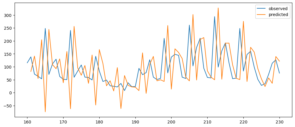
appendingTOR(tableOfResults, 'Ticket Sales', 'Autoregression', evaluateErrors(ticketSalesARResults))
tableOfResults| Unnamed: 0 | Data | Algorithm | MSE | RMSE | MAE |
|---|---|---|---|---|---|
| 1 | SP500 | Naive Forecasting | 0.315878 | 0.56203 | 0.325863 |
| 2 | FTSE | Naive Forecasting | 5.69646 | 2.38673 | 1.29783 |
| 3 | Gold | Naive Forecasting | 0.237289 | 0.487123 | 0.31245 |
| 4 | USDCUSDT Close Price | Naive Forecasting | 4.01536e-06 | 0.002004 | 0.001034 |
| 5 | USDCUSDT Tradecount | Naive Forecasting | 1.56376e+08 | 12505 | 7519.96 |
| 6 | Python Questions | Naive Forecasting | 1.00863e+06 | 1004.31 | 680.298 |
| 7 | Machine Learning Questions | Naive Forecasting | 3053.46 | 55.2581 | 35.4885 |
| 8 | Ticket Sales | Naive Forecasting | 12476 | 111.696 | 74.8537 |
| 9 | SP500 | Seasonal Forecasting - 60 | 24.0706 | 4.90618 | 3.19858 |
| 10 | SP500 | Seasonal Forecasting - 1440 | 578.648 | 24.0551 | 18.6964 |
| 11 | FTSE | Seasonal Forecasting - 60 | 358.944 | 18.9458 | 12.5549 |
| 12 | FTSE | Seasonal Forecasting - 1440 | 9305.27 | 96.4639 | 71.5358 |
| 13 | Gold | Seasonal Forecasting - 60 | 11.0817 | 3.32892 | 2.08104 |
| 14 | Gold | Seasonal Forecasting - 1440 | 297.39 | 17.245 | 12.2358 |
| 15 | USDCUSDT Close Price | Seasonal Forecasting | 1.41478e-05 | 0.003761 | 0.00176 |
| 16 | USDCUSDT Tradecount | Seasonal Forecasting | 2.76653e+08 | 16632.9 | 10558.5 |
| 17 | Python Questions | Seasonal Forecasting | 4.97505e+06 | 2230.48 | 1924.32 |
| 18 | Machine Learning Questions | Seasonal Forecasting | 14325.5 | 119.689 | 84.975 |
| 19 | Ticket Sales | Seasonal Forecasting | 3922.4 | 62.6291 | 37.0187 |
| 20 | SP500 | Average Forecasting - 60 | 8.21104 | 2.86549 | 1.84062 |
| 21 | SP500 | Average Forecasting - 1440 | 195.085 | 13.9673 | 10.6287 |
| 22 | FTSE | Average Forecasting - 60 | 122.369 | 11.0621 | 7.24807 |
| 23 | FTSE | Average Forecasting - 1440 | 3105.82 | 55.7299 | 40.9431 |
| 24 | Gold | Average Forecasting - 60 | 3.79681 | 1.94854 | 1.22559 |
| 25 | Gold | Average Forecasting - 1440 | 96.5074 | 9.82382 | 6.8452 |
| 26 | USDCUSDT Close Price | Average Forecasting | 6.51406e-06 | 0.002552 | 0.001187 |
| 27 | USDCUSDT Tradecount | Average Forecasting | 1.44419e+08 | 12017.5 | 7727.27 |
| 28 | Python Questions | Average Forecasting | 2.18019e+06 | 1476.55 | 1175.32 |
| 29 | Machine Learning Questions | Average Forecasting | 7140.3 | 84.5003 | 55.785 |
| 30 | Ticket Sales | Average Forecasting | 6061.2 | 77.8537 | 59.7301 |
| 31 | SP500 | Average Difference Forecasting - 60 | 0.322452 | 0.567849 | 0.332982 |
| 32 | SP500 | Average Difference Forecasting - 1440 | 0.316412 | 0.562505 | 0.326336 |
| 33 | FTSE | Average Difference Forecasting - 60 | 5.79875 | 2.40806 | 1.32178 |
| 34 | FTSE | Average Difference Forecasting - 1440 | 5.70723 | 2.38898 | 1.30033 |
| 35 | Gold | Average Difference Forecasting - 60 | 0.240423 | 0.49033 | 0.315994 |
| 36 | Gold | Average Difference Forecasting - 1440 | 0.237595 | 0.487437 | 0.313009 |
| 37 | USDCUSDT Close Price | Average Difference Forecasting | 4.53094e-06 | 0.002129 | 0.001103 |
| 38 | USDCUSDT Tradecount | Average Difference Forecasting | 1.64095e+08 | 12810 | 7724.69 |
| 39 | Python Questions | Average Difference Forecasting | 1.1445e+06 | 1069.81 | 751.801 |
| 40 | Machine Learning Questions | Average Difference Forecasting | 3399.79 | 58.3077 | 38.5563 |
| 41 | Ticket Sales | Average Difference Forecasting | 12936.3 | 113.738 | 76.6102 |
| 42 | SP500 | Naive Difference Forecasting | 0.553753 | 0.744146 | 0.456603 |
| 43 | FTSE | Naive Difference Forecasting | 10.796 | 3.28573 | 1.81081 |
| 44 | Gold | Naive Difference Forecasting | 0.521205 | 0.721946 | 0.480641 |
| 45 | USDCUSDT Close Price | Naive Difference Forecasting | 9.13676e-06 | 0.003023 | 0.001659 |
| 46 | USDCUSDT Tradecount | Naive Difference Forecasting | 4.15266e+08 | 20378.1 | 12089.8 |
| 47 | Python Questions | Naive Difference Forecasting | 2.34416e+06 | 1531.07 | 1117.71 |
| 48 | Machine Learning Questions | Naive Difference Forecasting | 6678.13 | 81.7198 | 51.9462 |
| 49 | Ticket Sales | Naive Difference Forecasting | 37594.4 | 193.893 | 136.398 |
| 50 | Gold | Autoregression | 0.167187 | 0.408885 | 0.270593 |
| 51 | SP500 | Autoregression | 0.181846 | 0.426434 | 0.236095 |
| 52 | Machine Learning Questions | Autoregression | 9493.88 | 97.4365 | 80.8513 |
| 53 | Ticket Sales | Autoregression | 12195.6 | 110.434 | 78.7188 |
Observations
tableOfResults[tableOfResults['Data'] == 'Machine Learning Questions'].sort_values('MSE')| Unnamed: 0 | Data | Algorithm | MSE | RMSE | MAE |
|---|---|---|---|---|---|
| 7 | Machine Learning Questions | Naive Forecasting | 3053.46 | 55.2581 | 35.4885 |
| 40 | Machine Learning Questions | Average Difference Forecasting | 3399.79 | 58.3077 | 38.5563 |
| 48 | Machine Learning Questions | Naive Difference Forecasting | 6678.13 | 81.7198 | 51.9462 |
| 29 | Machine Learning Questions | Average Forecasting | 7140.3 | 84.5003 | 55.785 |
| 52 | Machine Learning Questions | Autoregression | 9493.88 | 97.4365 | 80.8513 |
| 18 | Machine Learning Questions | Seasonal Forecasting | 14325.5 | 119.689 | 84.975 |
tableOfResults[tableOfResults['Data'] == 'Gold'].sort_values('MSE')| Unnamed: 0 | Data | Algorithm | MSE | RMSE | MAE |
|---|---|---|---|---|---|
| 50 | Gold | Autoregression | 0.167187 | 0.408885 | 0.270593 |
| 3 | Gold | Naive Forecasting | 0.237289 | 0.487123 | 0.31245 |
| 36 | Gold | Average Difference Forecasting - 1440 | 0.237595 | 0.487437 | 0.313009 |
| 35 | Gold | Average Difference Forecasting - 60 | 0.240423 | 0.49033 | 0.315994 |
| 44 | Gold | Naive Difference Forecasting | 0.521205 | 0.721946 | 0.480641 |
| 24 | Gold | Average Forecasting - 60 | 3.79681 | 1.94854 | 1.22559 |
| 13 | Gold | Seasonal Forecasting - 60 | 11.0817 | 3.32892 | 2.08104 |
| 25 | Gold | Average Forecasting - 1440 | 96.5074 | 9.82382 | 6.8452 |
| 14 | Gold | Seasonal Forecasting - 1440 | 297.39 | 17.245 | 12.2358 |
tableOfResults[tableOfResults['Data'] == 'SP500'].sort_values('MSE')| Unnamed: 0 | Data | Algorithm | MSE | RMSE | MAE |
|---|---|---|---|---|---|
| 51 | SP500 | Autoregression | 0.181846 | 0.426434 | 0.236095 |
| 1 | SP500 | Naive Forecasting | 0.315878 | 0.56203 | 0.325863 |
| 32 | SP500 | Average Difference Forecasting - 1440 | 0.316412 | 0.562505 | 0.326336 |
| 31 | SP500 | Average Difference Forecasting - 60 | 0.322453 | 0.567849 | 0.332982 |
| 42 | SP500 | Naive Difference Forecasting | 0.553753 | 0.744146 | 0.456603 |
| 20 | SP500 | Average Forecasting - 60 | 8.21104 | 2.86549 | 1.84062 |
| 9 | SP500 | Seasonal Forecasting - 60 | 24.0706 | 4.90618 | 3.19858 |
| 21 | SP500 | Average Forecasting - 1440 | 195.085 | 13.9673 | 10.6287 |
| 10 | SP500 | Seasonal Forecasting - 1440 | 578.648 | 24.0551 | 18.6964 |
tableOfResults[tableOfResults['Data'] == 'Ticket Sales'].sort_values('MSE')| Unnamed: 0 | Data | Algorithm | MSE | RMSE | MAE |
|---|---|---|---|---|---|
| 19 | Ticket Sales | Seasonal Forecasting | 3922.4 | 62.6291 | 37.0187 |
| 30 | Ticket Sales | Average Forecasting | 6061.2 | 77.8537 | 59.7301 |
| 53 | Ticket Sales | Autoregression | 12195.6 | 110.434 | 78.7188 |
| 8 | Ticket Sales | Naive Forecasting | 12476 | 111.696 | 74.8537 |
| 41 | Ticket Sales | Average Difference Forecasting | 12936.3 | 113.738 | 76.6102 |
| 49 | Ticket Sales | Naive Difference Forecasting | 37594.4 | 193.893 | 136.398 |
Simulated Trading
Let's try to apply the train_ar and predict from the lectures for the simulated trading. This will be heavily based off what is in the lectures.
def train_ar(values, order):
    target_vector = np.array(values[order:])
    lagged_values = []

    for i in range(len(values) - order):
        lagged_values.append(values[i:i+order])
    desgin_matrix = np.array(lagged_values)
    return np.linalg.inv(desgin_matrix.transpose() @ desgin_matrix) @ desgin_matrix.transpose() @ target_vector

def predict(coeffs, data):
    predicted_values = [math.nan] * len(coeffs)
    for i in range(len(coeffs), len(data)):
        predicted_values.append(np.dot(coeffs, data[i-len(coeffs):i]))
return np.array(predicted_values)goldData['Close'].plot()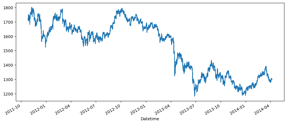
simTradingGoldData = goldData[goldData.index.dayofweek != 5]['Close'].sort_index()[:108000]
simTradingGoldData = pd.DataFrame(simTradingGoldData)
simTradingGoldData['Previous Close'] = simTradingGoldData['Close'].shift()
simTradingGoldData['Difference'] = simTradingGoldData['Close'] - simTradingGoldData['Close'].shift()

simTradingGoldData| ('Unnamed: 0_level_0', 'Datetime') | ('Close', 'Unnamed: 1_level_1') | ('Previous Close', 'Unnamed: 2_level_1') | ('Difference', 'Unnamed: 3_level_1') |
|---|---|---|---|
| 2011-10-26 15:50:00 | 1711.27 | nan | nan |
| 2011-10-26 15:51:00 | 1712.07 | 1711.27 | 0.80 |
| 2011-10-26 15:52:00 | 1712.13 | 1712.07 | 0.06 |
| 2011-10-26 15:53:00 | 1712.83 | 1712.13 | 0.70 |
| 2011-10-26 15:54:00 | 1713.87 | 1712.83 | 1.04 |
| ... | ... | ... | ... |
| 2012-02-15 01:19:00 | 1722.71 | 1723.55 | -0.84 |
| 2012-02-15 01:20:00 | 1722.79 | 1722.71 | 0.08 |
| 2012-02-15 01:21:00 | 1722.90 | 1722.79 | 0.11 |
| 2012-02-15 01:22:00 | 1722.86 | 1722.90 | -0.04 |
| 2012-02-15 01:23:00 | 1722.80 | 1722.86 | -0.06 |
trainingSimTradingGoldData = simTradingGoldData[:int(len(simTradingGoldData)*0.7)]
trainingSimTradingGoldData| ('Unnamed: 0_level_0', 'Datetime') | ('Close', 'Unnamed: 1_level_1') | ('Previous Close', 'Unnamed: 2_level_1') | ('Difference', 'Unnamed: 3_level_1') |
|---|---|---|---|
| 2011-10-26 15:50:00 | 1711.27 | nan | nan |
| 2011-10-26 15:51:00 | 1712.07 | 1711.27 | 0.80 |
| 2011-10-26 15:52:00 | 1712.13 | 1712.07 | 0.06 |
| 2011-10-26 15:53:00 | 1712.83 | 1712.13 | 0.70 |
| 2011-10-26 15:54:00 | 1713.87 | 1712.83 | 1.04 |
| ... | ... | ... | ... |
| 2012-01-12 17:32:00 | 1654.07 | 1653.40 | 0.67 |
| 2012-01-12 17:33:00 | 1653.85 | 1654.07 | -0.22 |
| 2012-01-12 17:34:00 | 1653.38 | 1653.85 | -0.47 |
| 2012-01-12 17:35:00 | 1653.46 | 1653.38 | 0.08 |
| 2012-01-12 17:36:00 | 1653.36 | 1653.46 | -0.10 |
testingSimTradingGoldData = simTradingGoldData[int(len(simTradingGoldData)*0.7):]
testingSimTradingGoldData| ('Unnamed: 0_level_0', 'Datetime') | ('Close', 'Unnamed: 1_level_1') | ('Previous Close', 'Unnamed: 2_level_1') | ('Difference', 'Unnamed: 3_level_1') |
|---|---|---|---|
| 2012-01-12 17:37:00 | 1653.12 | 1653.36 | -0.24 |
| 2012-01-12 17:38:00 | 1653.43 | 1653.12 | 0.31 |
| 2012-01-12 17:39:00 | 1653.20 | 1653.43 | -0.23 |
| 2012-01-12 17:40:00 | 1653.31 | 1653.20 | 0.11 |
| 2012-01-12 17:41:00 | 1652.87 | 1653.31 | -0.44 |
| ... | ... | ... | ... |
| 2012-02-15 01:19:00 | 1722.71 | 1723.55 | -0.84 |
| 2012-02-15 01:20:00 | 1722.79 | 1722.71 | 0.08 |
| 2012-02-15 01:21:00 | 1722.90 | 1722.79 | 0.11 |
| 2012-02-15 01:22:00 | 1722.86 | 1722.90 | -0.04 |
| 2012-02-15 01:23:00 | 1722.80 | 1722.86 | -0.06 |
plot_pacf(trainingSimTradingGoldData['Difference'].dropna())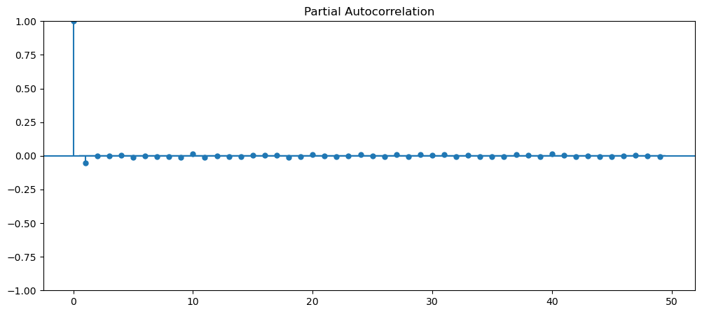

coeffs = train_ar(trainingSimTradingGoldData['Difference'].dropna(), 2)
coeffs
array([-0.00372669, -0.05243032])prediction = predict(coeffs, testingSimTradingGoldData['Difference'])
predictionarray([ nan, nan, -0.01535899, ..., -0.001064 ,
-0.00606547, 0.00168728])simTradingGoldDataResult = pd.DataFrame(testingSimTradingGoldData['Close'].rename('observed'))
simTradingGoldDataResult['predicted'] = prediction + testingSimTradingGoldData['Close']
simTradingGoldDataResult = simTradingGoldDataResult.dropna()
simTradingGoldDataResult.plot()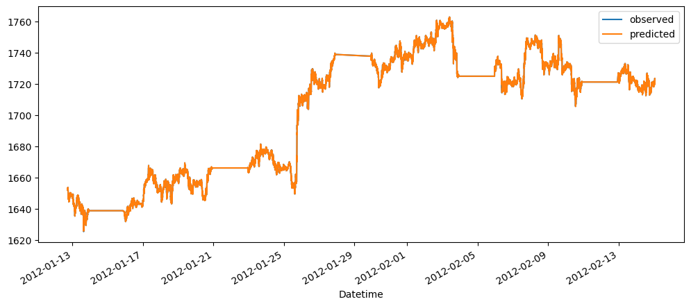
We will be using only 1.001 times larger than the previous. This is because when the value is 1.001, there are only 152 instances of True, and then at 1.002, there is only 8, and 1.003, there is only left with 4. That is why we proceeded to use 1.001
simTradingGoldDataResult['isHolding'] = simTradingGoldDataResult['predicted'] > simTradingGoldDataResult['observed'].shift() * 1.001
simTradingGoldDataResult[simTradingGoldDataResult['isHolding'] == True].count()
observed 152
predicted 152
isHolding 152
dtype: int64lastPrice = None
portfolioValue = 10000
values = []
for ts, (close, _, isHolding) in simTradingGoldDataResult.iterrows():
if isHolding:
portfolioValue *= close / lastPrice
lastPrice = close
values.append(portfolioValue)
simTradingGoldDataResult['Equity Value'] = valuesoffsets = (simTradingGoldDataResult['isHolding'] * (simTradingGoldDataResult['observed'].shift(-1) - simTradingGoldDataResult['observed']))
hasIncreased = ((simTradingGoldDataResult['observed'].shift(-1) > simTradingGoldDataResult['observed']) & simTradingGoldDataResult['isHolding']).astype(int)
hasDecreased = ((simTradingGoldDataResult['observed'].shift(-1) < simTradingGoldDataResult['observed']) & simTradingGoldDataResult['isHolding']).astype(int)
plt.figure()
ax = simTradingGoldDataResult['observed'].plot()
for no, i in enumerate(hasIncreased):
if i:
plt.axvline(hasIncreased.index[no], color='g', linewidth=0.3)
for no, i in enumerate(hasDecreased):
if i:
plt.axvline(hasIncreased.index[no], color='r', linewidth=0.3)
plt.show()
for no, i in enumerate(hasIncreased):
if i:
plt.axvline(hasIncreased.index[no], color='g', linewidth=0.3)
for no, i in enumerate(hasDecreased):
if i:
plt.axvline(hasIncreased.index[no], color='r', linewidth=0.3)
simTradingGoldDataResult['Equity Value'].plot()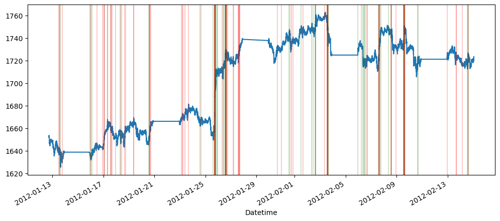
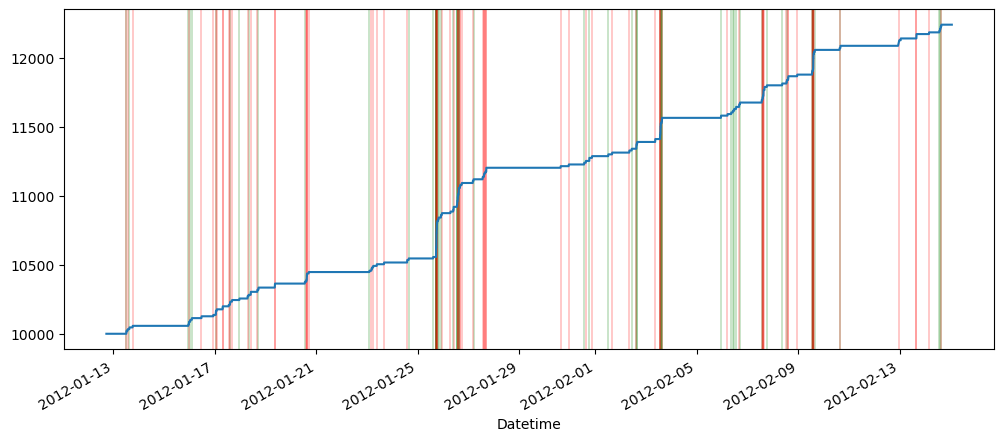
Monte Carlo Simulations
We will now apply Monte Carlo to 3 datasets and explore. We will be using the gold data (for its real-worldness), machine learning questions (for its multiplicative graph), and ticket sales (for its seasonality). Furthermore, using the result found from PACF above. We can use the similar concept above, were we split the training and testing set.
Gold
def mcRmse(predicted, actual):
    diffs = predicted - actual
    return math.sqrt(np.mean(diffs**2))
goldTrainSeries = goldData.reset_index()['Close'][:traniningStationaryGoldDataLength]
goldTrainSeries0 1298.50
1 1298.60
2 1298.90
3 1299.09
4 1299.17
...
75595 1246.30
75596 1246.60
75597 1246.40
75598 1247.10
75599 1247.20
Name: Close, Length: 75600, dtype: float64goldModel = AutoReg(goldTrainSeries, 3, trend='n').fit()
goldCoeffs = list(reversed(goldModel.params))
goldCoeffs[0.032491603321171736, 0.12017858859369826, 0.8473291714654028]goldStdDev = mcRmse(goldModel.predict(), goldTrainSeries)
goldStdDev0.36114889408159995numOfSamplesGold = 1000
goldTestSeries = goldData.reset_index()['Close'][traniningStationaryGoldDataLength:stationaryGoldDataLength]
goldTestSeries = goldTestSeries.reset_index()['Close']
initialGoldValues = np.array(goldTestSeries[:2500]).reshape(1, -1)
initialGoldValues
goldValues = np.broadcast_to(initialGoldValues, (numOfSamplesGold, 2500))
goldValues
goldTrajectoryLength = 1000
np.random.seed(123)
for i in range(goldTrajectoryLength):
nextPrediction = goldValues[:, -3:] @ goldCoeffs
nextColumn = nextPrediction + goldStdDev * np.random.randn(numOfSamplesGold)
goldValues = np.append(goldValues, nextColumn.reshape(numOfSamplesGold, 1), axis = 1)
horizontalLines = [x for x in range(1220, 1281, 10)]
plt.plot(goldValues.transpose())
for line in horizontalLines:
plt.axhline(y = line, linestyle = 'dashed', linewidth = 2, alpha = 0.5)
plt.plot(goldTestSeries[:3500], linewidth = 1.5, c = 'black')
plt.show()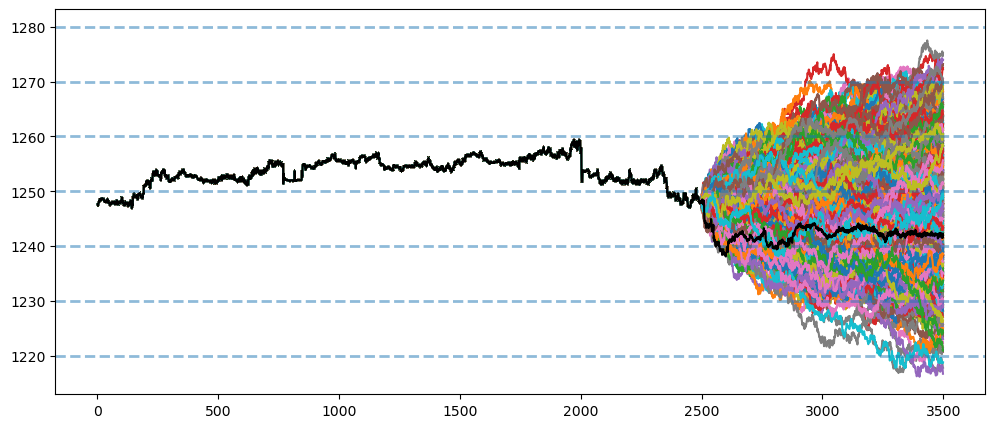
Now that we have produced a 1000 samples of possible price movements, we can now calculate the difference probabilities of it reaching certain prices and what not.
The black line shown in the plot, is to show the actual gold price move.
finalTimePeriod = nextColumn
finalTimePeriod
array([1248.81453198, 1234.48618073, 1260.43243186, 1249.37824546,
1246.44648938, 1234.98845302, 1237.40624842, 1263.51763179,
1249.32173509, 1237.21926607, 1262.02420909, 1241.23580835,
...
1255.65131606, 1269.97946134, 1258.23988999, 1249.41256685])We can look into what are the probabilities of the price of gold to reach a certain price at time 3500. Using the function from the materials given, we can calculate the probability.
def probBetween (arr, lower, higher):
    count = np.count_nonzero((arr > lower) & (arr < higher))
    return count/arr.size
The probability of the gold of price reaching between 1220 to 1280
probBetween(finalTimePeriod, 1220, 1280)0.997The probability of the gold of price reaching between 1215 and 1240
probBetween(finalTimePeriod, 1215, 1240)0.231The probability of the gold of price reaching between 1245 and 1255
probBetween(finalTimePeriod, 1245, 1255)0.36The probability of the gold of price reaching between 1245 and 1255
probBetween(finalTimePeriod, 1250, 1260)0.296The probability of the gold of price reaching between 1265 and 1280
probBetween(finalTimePeriod, 1265, 1280)0.042The probability of the gold of price reaching between 1250 and 1253
probBetween(finalTimePeriod, 1250, 1253)0.101The further away in the future we try to predict, the harder it is to determine the prices, and because the cone of possibility is larger, many prices that we set out to find, have generally the same probability. The lower it is further away from the first prediction value.
Next, we will look into the probability that the price will go beyond or lower than a specific value. Let's say we would like to find out if there are any higher probability of either direction, and then we will try some other values instead.
# Checking if calling the correct
goldValues[:,2500][:5]
array([1247.77539526, 1248.52765975, 1248.26966692, 1247.62347288,
1247.95850871])goldValues[:,2499][:5]array([1248.2, 1248.2, 1248.2, 1248.2, 1248.2])period = 2499
lastPrice = goldValues[:,period][0]
lastPrice1248.2(lastPrice < goldValues[:,2500:]).sum() / (numOfSamplesGold*goldTrajectoryLength)0.487236(lastPrice > goldValues[:,2500:]).sum() / (numOfSamplesGold*goldTrajectoryLength)0.512764Based on the monte carlo result, there are 45.23% of values that are larger the last point we were and 54.73% of them are lower. Because of that, let's assume we enter a short position, now lets explore further in time of our result.
Let's say we are now we would like to only hold on to the position only for a shorter term. At period 2750, we would like to exit the position. What are the probability of it to take profit on 1240, or stop loss on 1260, or let's be conservative and also find out the probability for it at 1255.
takeProfit = 1240
np.any(takeProfit > goldValues[:,2500:2750], axis = 1).sum() / 10000.088stopLoss = 1260
np.any(stopLoss < goldValues[:,2500:2750], axis = 1).sum() / 10000.008conservativeStopLoss = 1255
np.any(conservativeStopLoss < goldValues[:,2500:2750], axis = 1).sum() / 10000.145Given that the chances for the price of 1255 is higher than the initial take profit of 1240, we might want to adjust it lower to increase our chances to trigger the take profit.
takeProfit = 1240.5
np.any(takeProfit > goldValues[:,2500:2750], axis = 1).sum() / 10000.109takeProfit = 1241.5
np.any(takeProfit > goldValues[:,2500:2750], axis = 1).sum() / 10000.168By increasing the stop loss by 0.5, we have increased the probability of to 0.144, and be more conservative, at 1241.5, the chances for us to increased to 0.205.
The following is the density plot for the gold values.
xTicks = [x for x in range(1190, 1311, 10)]
goldValuesSumKDE = []
for i in goldValues:
    [goldValuesSumKDE.append(x) for x in i[2500:]]
pd.DataFrame(goldValuesSumKDE).plot.kde()
plt.axvline(lastPrice, linestyle = 'dashed', label = 'Last Price', c = 'black')
plt.xticks(xTicks)
for line in xTicks:
    plt.axvline(line, linestyle = 'dotted', c = 'b', alpha = 0.3)
plt.legend()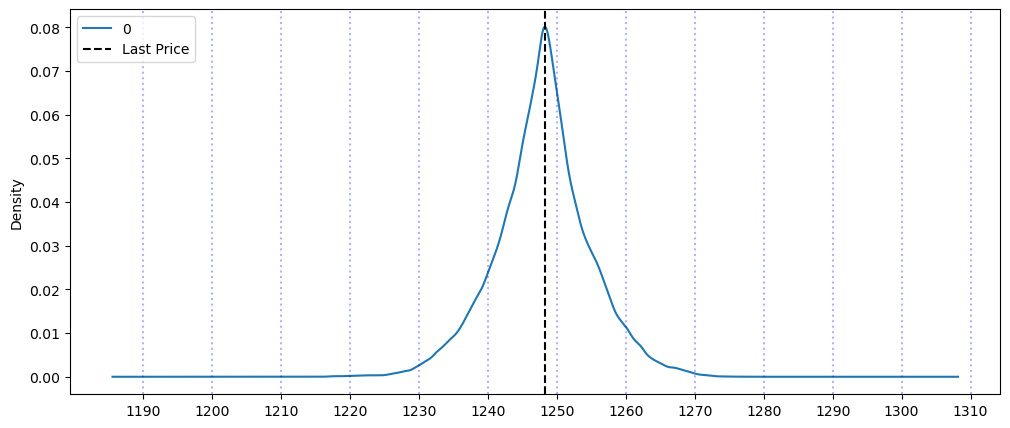
The following is the density plot for period from 2500 to 2750, according to the scenario above. Here, we can visualize its probability of each given range of prices, based on the monte carlo results. As we can see that, a small increase from 1240, would significantly increase the probability as shown in the steep increase.
xTicks = [x for x in range(1190, 1311, 10)]
goldValuesSumKDE = []
for i in goldValues:
    [goldValuesSumKDE.append(x) for x in i[2500:2750]]
pd.DataFrame(goldValuesSumKDE).plot.kde()
plt.axvline(lastPrice, linestyle = 'dashed', label = 'Last Price', c = 'black')
plt.xticks(xTicks)
for line in xTicks:
    plt.axvline(line, linestyle = 'dotted', c = 'b', alpha = 0.3)
plt.legend()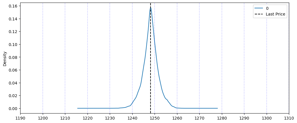
Cinema Tickets
Given the time contraints on working on the coursework, we will explore one more datasaet before moving on.
ticketSalesTrainSeries = ticketSales_data['tickets_sold'].reset_index()['tickets_sold'][:trainingStationaryTicketSales]
ticketSalesTrainSeries
0 125.650000
1 178.675325
2 175.461017
3 114.192192
4 94.831956
...
156 73.299830
157 71.350000
158 275.887784
159 148.436834
160 115.308869
Name: tickets_sold, Length: 161, dtype: float64ticketSalesModel = AutoReg(ticketSalesTrainSeries, 7, trend='n').fit()
ticketSalesCoeffs = list(reversed(ticketSalesModel.params))
ticketSalesCoeffs[0.7426181566741853,
-0.03903937266016291,
-0.031596445533128875,
0.036661173670043956,
0.10106447839651159,
0.0957974652301363,
0.08677635276613055]ticketsSalesStdDev = mcRmse(ticketSalesModel.predict(), ticketSalesTrainSeries)
ticketsSalesStdDev62.78175334614299numOfSamplesTicketSales = 71 - 14def runMonteCarloTicketSale(multiplier):
np.random.seed(123)
ticketSalesTestSeries = ticketSales_data['tickets_sold'].reset_index()['tickets_sold'][trainingStationaryTicketSales:]
ticketSalesTestSeries = ticketSalesTestSeries.reset_index()['tickets_sold']
initialTicketSalesValues = np.array(ticketSalesTestSeries[:14]).reshape(1, -1)
ticketSalesValues = np.broadcast_to(initialTicketSalesValues, (numOfSamplesTicketSales, 14))
ticketSalesTrajectoryLength = (71 - 14)
for i in range(ticketSalesTrajectoryLength):
nextPrediction = ticketSalesValues[:, -7:] @ ticketSalesCoeffs
nextColumn = nextPrediction + multiplier * np.random.randn(numOfSamplesTicketSales)
ticketSalesValues = np.append(ticketSalesValues, nextColumn.reshape(numOfSamplesTicketSales, 1), axis = 1)
horizontalLines = [x for x in range(-300, 501, 100)]
plt.plot(ticketSalesValues.transpose())
for line in horizontalLines:
plt.axhline(y = line, linestyle = 'dashed', linewidth = 2, alpha = 0.5)
plt.plot(ticketSalesTestSeries[:71], linewidth = 1.5, c = 'black')
plt.yticks(horizontalLines)
plt.show()runMonteCarloTicketSale(ticketsSalesStdDev)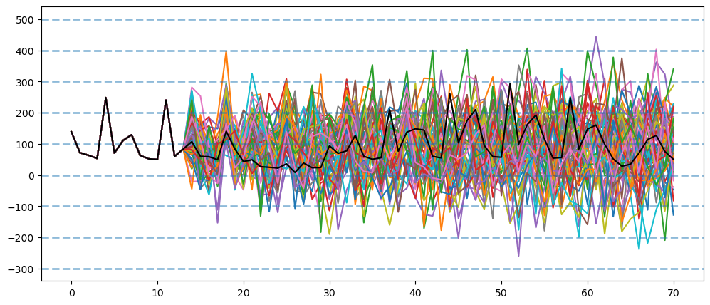
After visualizing the monte carlo simulation, realized that it might not be suitable for ths dataset because, the random nature of the monte carlo will include predictions of negative number, when this dataset will not ever reach so. Then, I thought what if we were to use other values rather than the standard deviations, such as the ones shown below. The above def/function was implemented after the realization.
Using several values and test to see how the results would be
runMonteCarloTicketSale(10)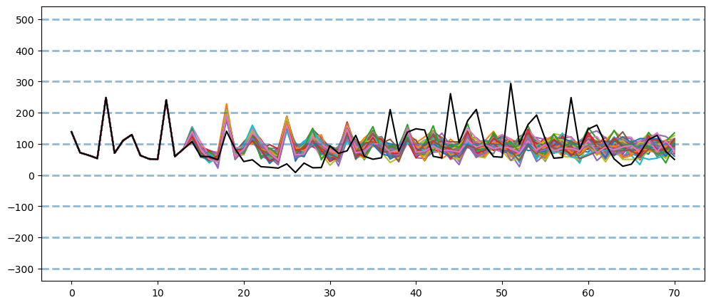
runMonteCarloTicketSale(30)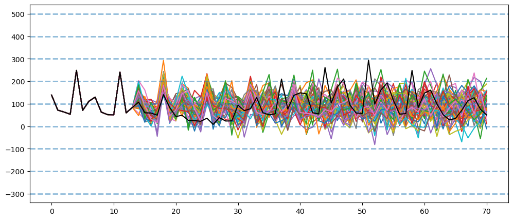
runMonteCarloTicketSale(10 + np.random.randint(10, ticketsSalesStdDev))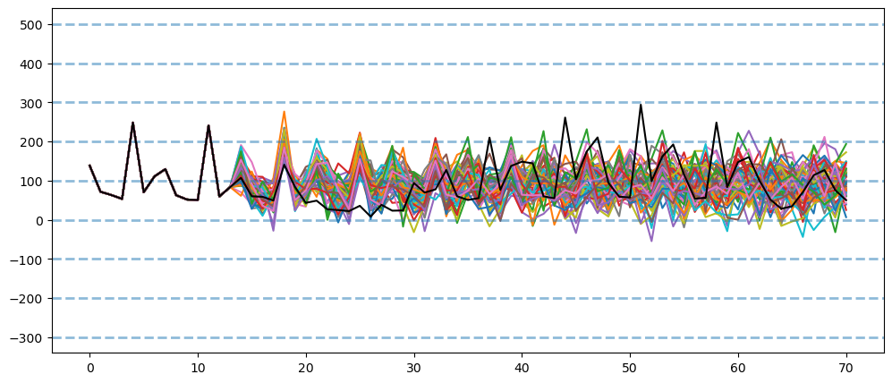
We even have tried using a varying value with the last one, but they all seem to have predictions being too narrow and might shrink even more if further in time. So next we will try removing 0 and below, but using the abs() function
def runMonteCarloTicketSale2(multiplier):
    np.random.seed(123)
    ticketSalesTestSeries = ticketSales_data['tickets_sold'].reset_index()['tickets_sold'][trainingStationaryTicketSales:]
    ticketSalesTestSeries = ticketSalesTestSeries.reset_index()['tickets_sold']

    initialTicketSalesValues = np.array(ticketSalesTestSeries[:14]).reshape(1, -1)

    ticketSalesValues = np.broadcast_to(initialTicketSalesValues, (numOfSamplesTicketSales, 14))

    ticketSalesTrajectoryLength = (71 - 14)

    for i in range(ticketSalesTrajectoryLength):
        nextPrediction = ticketSalesValues[:, -7:] @ ticketSalesCoeffs
        nextColumn = nextPrediction + abs(multiplier * np.random.randn(numOfSamplesTicketSales))
        ticketSalesValues = np.append(ticketSalesValues, nextColumn.reshape(numOfSamplesTicketSales, 1), axis = 1)

    horizontalLines = [x for x in range(-300, 501, 100)]

    plt.plot(ticketSalesValues.transpose())
    for line in horizontalLines:
        plt.axhline(y = line, linestyle = 'dashed', linewidth = 2, alpha = 0.5)
    plt.plot(ticketSalesTestSeries[:71], linewidth = 1.5, c = 'black')
    plt.yticks(horizontalLines)
plt.show()runMonteCarloTicketSale2(ticketsSalesStdDev)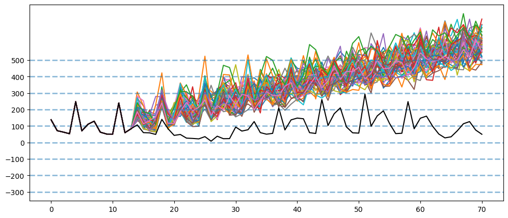
By only having positive numbers, it somehow affected the prediction to only trend upwards, which is also not ideal either.
Regardless of which parameter used, it does seem that the model, given for this dataset, work best only at the first few period. While monte carlo simulation was supposed to be able to solve this issue, but it does not. While it is very useful to be used as a baseline, to understand the possible and very probable outcomes, and to have a probabilistic view of the upcoming time frames, it quickly becomes unreliable too far in the future, similar to many models.
Moving Averages
def maSmoothing(series, n):
    answer = series - series
    for i in range(n):
        answer = answer + series.shift(i)
    return answer/n

def maSmoothingPlot(series, nList):
    temp = pd.Series(series, name='observed')
    temp = pd.DataFrame(temp)
    for i in nList:
        tempCol = 'smoothed ' + str(i)
        temp[tempCol] = maSmoothing(temp['observed'], i)

    return temp
Gold
maSmoothingPlot(goldData['Close'][:3000], [10,100,500]).plot()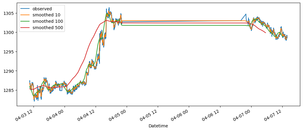
FTSE
maSmoothingPlot(ftseData['Close'][:100000], [100,3000,10000]).plot()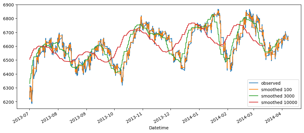
S&P500
maSmoothingPlot(sp500Data['Close'][:100000], [500,5000,10000]).plot()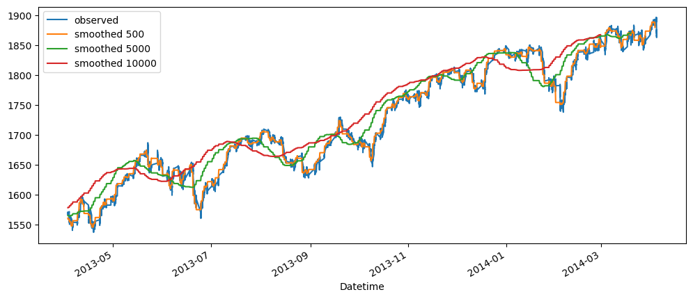
USDCUSDT - Tradecount
maSmoothingPlot(usdcusdtDataTradeCount['tradecount'].sort_index(),[10,50,100]).plot()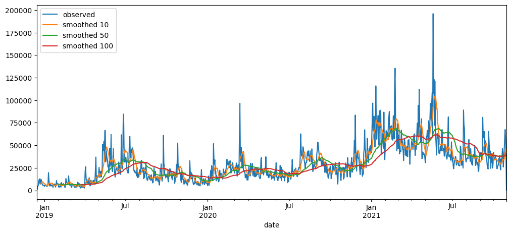
Cinema Tickets
maSmoothingPlot(ticketSales_data['tickets_sold'], [3,7,21]).plot()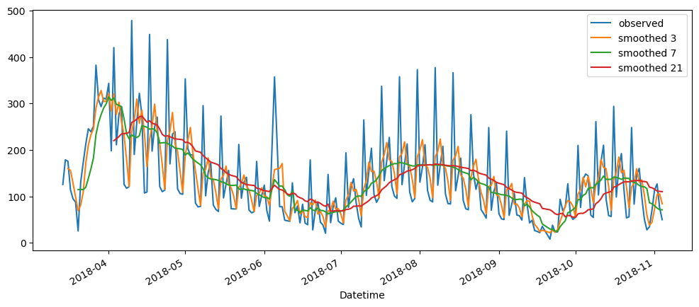
Machine Learning Questions
maSmoothingPlot(mlStackoverflow_data['machine-learning'], [3,7,20]).plot()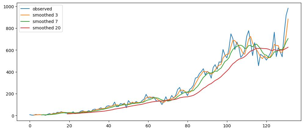
Moving average is a very equal and simple way to get an sense of the trending within the data. The downside of moving averages is that if there is not enough data for a longer time frame period, we need to wait however the selected period is, for the data to finalize. While there are many longer term investing strategies that utilizes the moving average, they are usually implemented for trend finding. Another downside is that, we will need to sacrifice some data, usually in the front of the dataset, to be used for the calculation of the average. The dataset will suffer a little from that chunk of missing data
Exponential Averaging
The following averaging method is interesting because it does not need to wait for a given period. However, we do need set a parameter, which will affect the how smooth the line is. Similarly, we will explore this will all the datasets.
def expSmoothing (series, alpha):
    smoothedValue = series[0]
    results = []
    for value in series:
        smoothedValue = (1 - alpha) * smoothedValue + alpha * value
        results.append(smoothedValue)
    return results

def expSmoothingPlot (series, list):
    temp = pd.Series(series, name='observed')
    temp = pd.DataFrame(temp)
    for n in list:
        tempCol = 'smoothed ' + str(n)
        temp[tempCol] = expSmoothing(temp['observed'], n)
    return temp
Gold
expSmoothingPlot(goldData['Close'][:3000], [0.9, 0.05, 0.01, 0.003]).plot()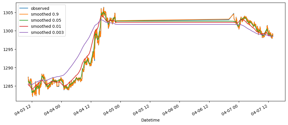
FTSE
expSmoothingPlot(ftseData['Close'][:100000], [0.0005, 0.0001]).plot()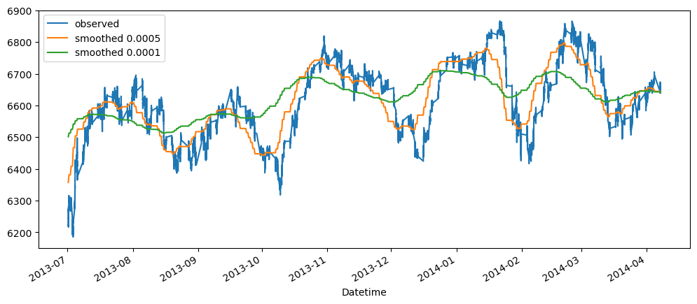
S&P500
expSmoothingPlot(sp500Data['Close'][:100000], [0.0024, 0.0005, 0.0001]).plot()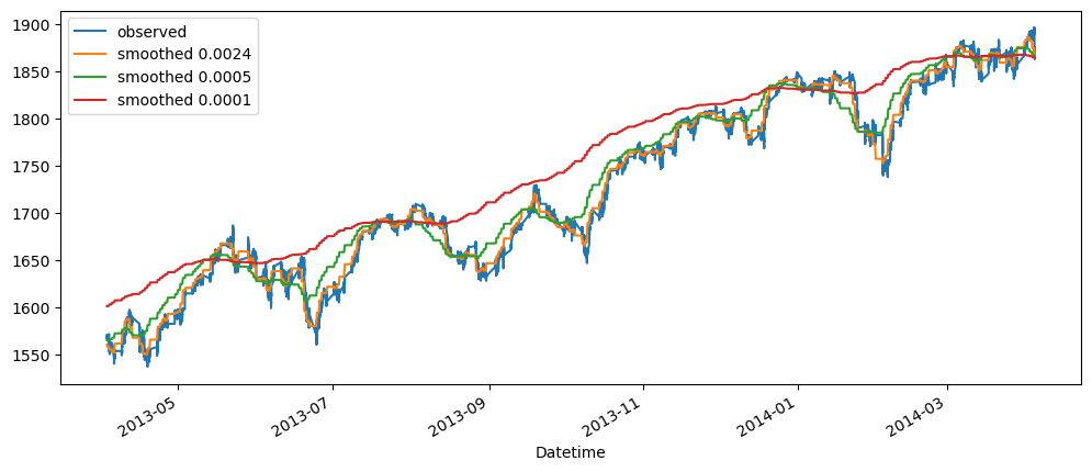
USDCUSDT - Tradecount
expSmoothingPlot(usdcusdtDataTradeCount['tradecount'].sort_index(), [0.1, 0.01, 0.001]).plot()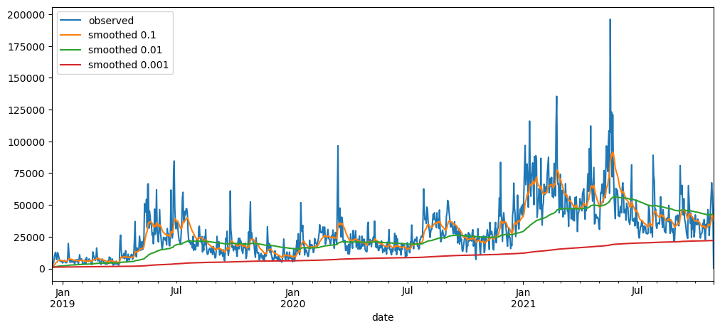
Cinema Tickets
expSmoothingPlot(ticketSales_data['tickets_sold'], [0.1, 0.05, 0.025, 0.01]).plot()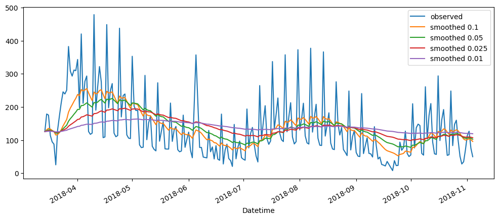
Machine Learning Questions
expSmoothingPlot(mlStackoverflow_data['machine-learning'], [0.25, 0.1, 0.01]).plot()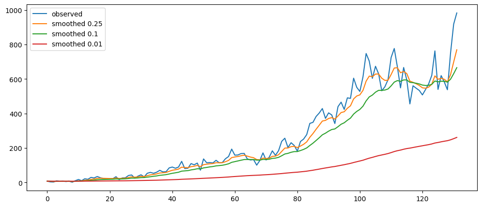
Based on the above, we can see that the alpha number, really largely depends on the size of the dataset. 0.1 on one mimics the graph very closely while on the other, it is already near a straight line.
Removing Trend with EMA
The good thing about using EMA, is that the first few values of the dataset will not be excluded, making it easier for us to remove the trend portion of the dataset. Then, it should become stationary. We can also test the stationarity of the data with the kpss and adf test. We wil then explore if it predicts better this way.
We will only do one dataset to explore given the limited time.
First, we will need to see which value of alpha produces the most stationary graph. We will be decide it visually, only then we check with the tests
emaGoldData = expSmoothingPlot(goldData['Close'][:stationaryGoldDataLength], [0.001, 0.005, 0.0002])emaGoldData.columnsIndex(['observed', 'smoothed 0.001', 'smoothed 0.005', 'smoothed 0.0002'], dtype='object')for i in range(1,4):
currentCol = emaGoldData.columns[i]
smoothed = emaGoldData[currentCol]
plt.plot(emaGoldData['observed'] - smoothed, label = currentCol, alpha=0.7)
plt.legend()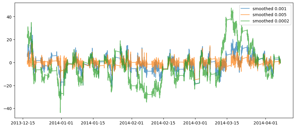
Visually, we can see that the alpha value of 0.005, seem to be a good fit for this case. So we will be using it.
emaGoldData['residual'] = emaGoldData['observed'] - emaGoldData['smoothed 0.005']kpss_test(emaGoldData['residual'])KPSS Stat: 0.4907302016778367
p-value: 0.04375445908156831
Number of lags: 192
Critial Values:
10% : 0.347
5% : 0.463
2.5% : 0.574
1% : 0.739
Result: The series is not stationaryadftest(emaGoldData['residual'])AdfTest Stat: -16.70183985809975
p-value: 1.4590092692087397e-29
Number of lags: 50
Number of observation: 107949
Critial Values:
1% : -3.430410579120753
5% : -2.8615667750440084
10% : -2.5667842514152195
The series is stationaryVisually, it might look like the data is already stationary, but based on two tests, it is still not the case. Therefore, we can try to proceed with getting the difference.
emaGoldData['residualDiff'] = emaGoldData['residual'] - emaGoldData['residual'].shift()
emaGoldData[['residual', 'residualDiff']].plot()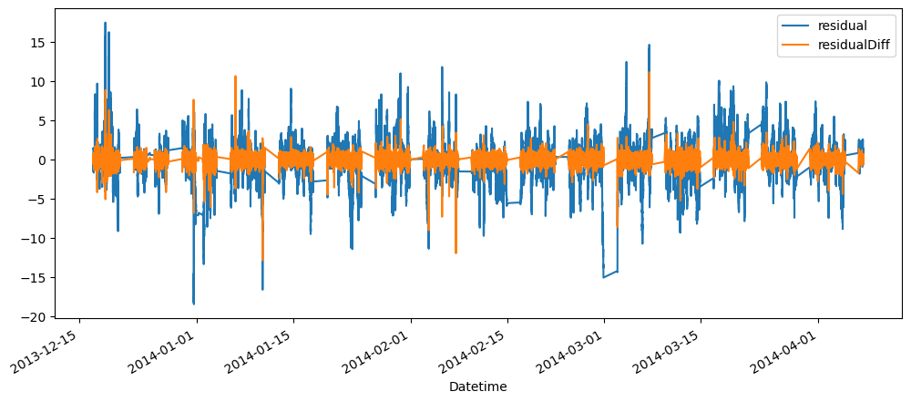
kpss_test(emaGoldData['residualDiff'][1:])KPSS Stat: 0.0010710001653877659
p-value: 0.1
Number of lags: 71
Critial Values:
10% : 0.347
5% : 0.463
2.5% : 0.574
1% : 0.739
Result: The series is stationaryadftest(emaGoldData['residualDiff'][1:])AdfTest Stat: -47.34320740713912
p-value: 0.0
Number of lags: 53
Number of observation: 107945
Critial Values:
1% : -3.4304105813656207
5% : -2.8615667760361956
10% : -2.5667842519433277
The series is stationaryNow we will proceed with applying prediction methods.
plot_pacf(emaGoldData['residualDiff'][1:traniningStationaryGoldDataLength])
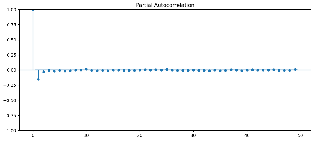
Seem like only the 2nd period is effective, however, let's just use a bigger scale period.
emaGoldCoeffs = train_ar(emaGoldData['residualDiff'][1:traniningStationaryGoldDataLength],20)
emaGoldCoeffs
array([ 0.00133632, -0.00681158, -0.006989 , -0.00519191, -0.00436599,
-0.00034325, -0.01157953, -0.00883011, -0.01158689, -0.00957072,
0.01358625, 0.00297729, -0.00152516, -0.01193093, -0.01983785,
-0.01051143, -0.02078453, -0.0104172 , -0.03703278, -0.15587259])emaGoldResidualDiffPredict = predict(emaGoldCoeffs, emaGoldData['residualDiff'][traniningStationaryGoldDataLength:] )
emaGoldResidualDiffPredict = pd.DataFrame(emaGoldResidualDiffPredict)
emaGoldResidualDiffPredict = emaGoldResidualDiffPredict.set_index(pd.Series([x for x in range(traniningStationaryGoldDataLength,stationaryGoldDataLength)]))
emaGoldResidualDiffPredict.plot()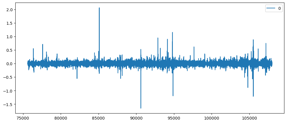
emaGoldResidualPrediction = emaGoldResidualDiffPredict[0] + emaGoldData.reset_index()['residualDiff'][traniningStationaryGoldDataLength:].shift()
emaGoldResidualPrediction.plot()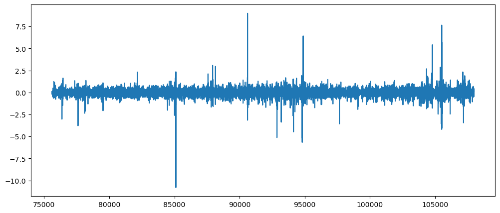
emaGoldTrendPredict = 2 * emaGoldData['smoothed 0.005'][traniningStationaryGoldDataLength:].shift(1) \
- emaGoldData['smoothed 0.005'][traniningStationaryGoldDataLength:].shift(2)
emaGoldTrendPredict = pd.DataFrame(emaGoldTrendPredict.reset_index()['smoothed 0.005'].rename('trend prediction'))\
.set_index(pd.Series([x for x in range(traniningStationaryGoldDataLength, stationaryGoldDataLength)]))
emaGoldTrendPredict.plot()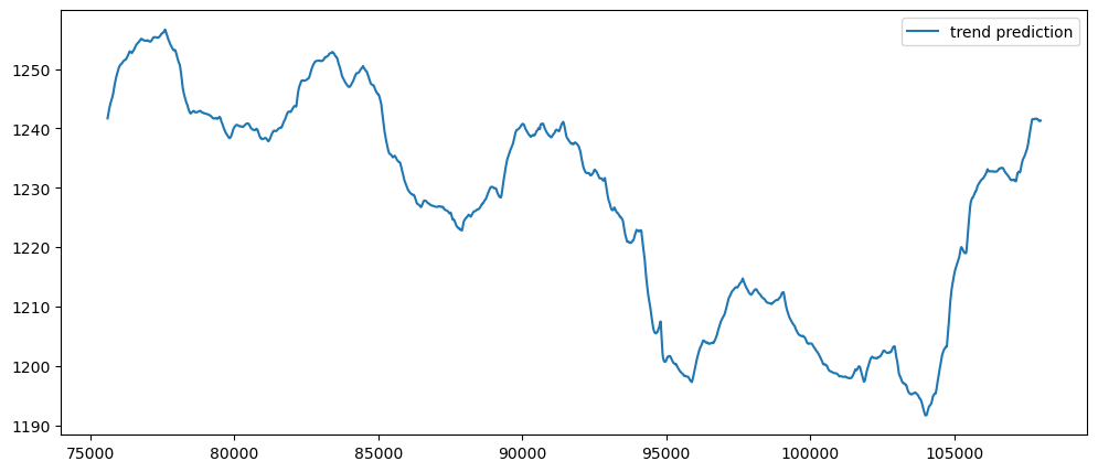
emaGoldPrediction = emaGoldTrendPredict['trend prediction'] + emaGoldResidualPrediction
emaGoldResult = pd.DataFrame(emaGoldData.reset_index()['observed'][traniningStationaryGoldDataLength:])
emaGoldResult['predicted'] = emaGoldPrediction
emaGoldResult = emaGoldResult.dropna()
emaGoldResult.plot()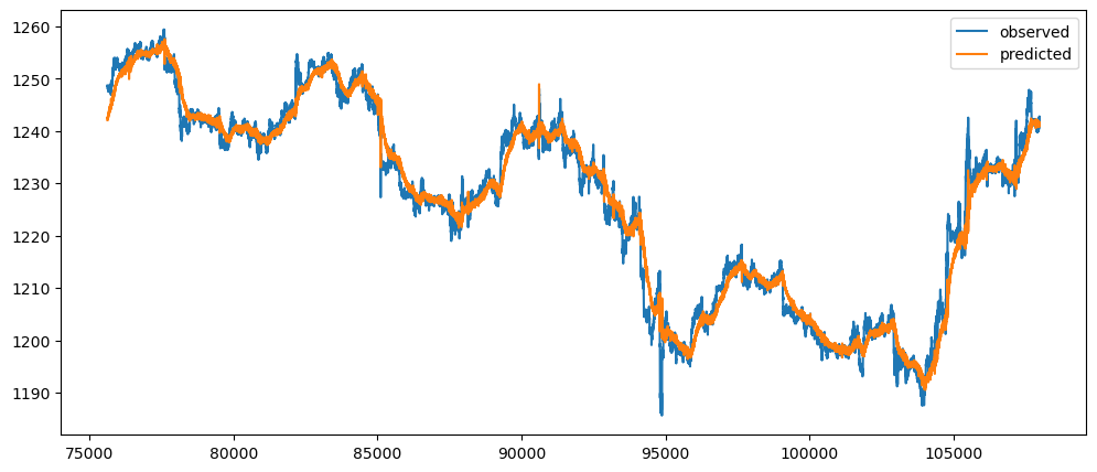
evaluateErrors(emaGoldResult)[8.310943507413699, 2.882870705982788, 1.9945175517858817]appendingTOR(tableOfResults, 'Gold', 'Manual ARIMA',evaluateErrors(emaGoldResult))
tableOfResults| Unnamed: 0 | Data | Algorithm | MSE | RMSE | MAE |
|---|---|---|---|---|---|
| 1 | SP500 | Naive Forecasting | 0.315878 | 0.56203 | 0.325863 |
| 2 | FTSE | Naive Forecasting | 5.69646 | 2.38673 | 1.29783 |
| 3 | Gold | Naive Forecasting | 0.237289 | 0.487123 | 0.31245 |
| 4 | USDCUSDT Close Price | Naive Forecasting | 4.01536e-06 | 0.002004 | 0.001034 |
| 5 | USDCUSDT Tradecount | Naive Forecasting | 1.56376e+08 | 12505 | 7519.96 |
| 6 | Python Questions | Naive Forecasting | 1.00863e+06 | 1004.31 | 680.298 |
| 7 | Machine Learning Questions | Naive Forecasting | 3053.46 | 55.2581 | 35.4885 |
| 8 | Ticket Sales | Naive Forecasting | 12476 | 111.696 | 74.8537 |
| 9 | SP500 | Seasonal Forecasting - 60 | 24.0706 | 4.90618 | 3.19858 |
| 10 | SP500 | Seasonal Forecasting - 1440 | 578.648 | 24.0551 | 18.6964 |
| 11 | FTSE | Seasonal Forecasting - 60 | 358.944 | 18.9458 | 12.5549 |
| 12 | FTSE | Seasonal Forecasting - 1440 | 9305.27 | 96.4639 | 71.5358 |
| 13 | Gold | Seasonal Forecasting - 60 | 11.0817 | 3.32892 | 2.08104 |
| 14 | Gold | Seasonal Forecasting - 1440 | 297.39 | 17.245 | 12.2358 |
| 15 | USDCUSDT Close Price | Seasonal Forecasting | 1.41478e-05 | 0.003761 | 0.00176 |
| 16 | USDCUSDT Tradecount | Seasonal Forecasting | 2.76653e+08 | 16632.9 | 10558.5 |
| 17 | Python Questions | Seasonal Forecasting | 4.97505e+06 | 2230.48 | 1924.32 |
| 18 | Machine Learning Questions | Seasonal Forecasting | 14325.5 | 119.689 | 84.975 |
| 19 | Ticket Sales | Seasonal Forecasting | 3922.4 | 62.6291 | 37.0187 |
| 20 | SP500 | Average Forecasting - 60 | 8.21104 | 2.86549 | 1.84062 |
| 21 | SP500 | Average Forecasting - 1440 | 195.085 | 13.9673 | 10.6287 |
| 22 | FTSE | Average Forecasting - 60 | 122.369 | 11.0621 | 7.24807 |
| 23 | FTSE | Average Forecasting - 1440 | 3105.82 | 55.7299 | 40.9431 |
| 24 | Gold | Average Forecasting - 60 | 3.79681 | 1.94854 | 1.22559 |
| 25 | Gold | Average Forecasting - 1440 | 96.5074 | 9.82382 | 6.8452 |
| 26 | USDCUSDT Close Price | Average Forecasting | 6.51406e-06 | 0.002552 | 0.001187 |
| 27 | USDCUSDT Tradecount | Average Forecasting | 1.44419e+08 | 12017.5 | 7727.27 |
| 28 | Python Questions | Average Forecasting | 2.18019e+06 | 1476.55 | 1175.32 |
| 29 | Machine Learning Questions | Average Forecasting | 7140.3 | 84.5003 | 55.785 |
| 30 | Ticket Sales | Average Forecasting | 6061.2 | 77.8537 | 59.7301 |
| 31 | SP500 | Average Difference Forecasting - 60 | 0.322452 | 0.567849 | 0.332982 |
| 32 | SP500 | Average Difference Forecasting - 1440 | 0.316412 | 0.562505 | 0.326336 |
| 33 | FTSE | Average Difference Forecasting - 60 | 5.79875 | 2.40806 | 1.32178 |
| 34 | FTSE | Average Difference Forecasting - 1440 | 5.70723 | 2.38898 | 1.30033 |
| 35 | Gold | Average Difference Forecasting - 60 | 0.240423 | 0.49033 | 0.315994 |
| 36 | Gold | Average Difference Forecasting - 1440 | 0.237595 | 0.487437 | 0.313009 |
| 37 | USDCUSDT Close Price | Average Difference Forecasting | 4.53094e-06 | 0.002129 | 0.001103 |
| 38 | USDCUSDT Tradecount | Average Difference Forecasting | 1.64095e+08 | 12810 | 7724.69 |
| 39 | Python Questions | Average Difference Forecasting | 1.1445e+06 | 1069.81 | 751.801 |
| 40 | Machine Learning Questions | Average Difference Forecasting | 3399.79 | 58.3077 | 38.5563 |
| 41 | Ticket Sales | Average Difference Forecasting | 12936.3 | 113.738 | 76.6102 |
| 42 | SP500 | Naive Difference Forecasting | 0.553753 | 0.744146 | 0.456603 |
| 43 | FTSE | Naive Difference Forecasting | 10.796 | 3.28573 | 1.81081 |
| 44 | Gold | Naive Difference Forecasting | 0.521205 | 0.721946 | 0.480641 |
| 45 | USDCUSDT Close Price | Naive Difference Forecasting | 9.13676e-06 | 0.003023 | 0.001659 |
| 46 | USDCUSDT Tradecount | Naive Difference Forecasting | 4.15266e+08 | 20378.1 | 12089.8 |
| 47 | Python Questions | Naive Difference Forecasting | 2.34416e+06 | 1531.07 | 1117.71 |
| 48 | Machine Learning Questions | Naive Difference Forecasting | 6678.13 | 81.7198 | 51.9462 |
| 49 | Ticket Sales | Naive Difference Forecasting | 37594.4 | 193.893 | 136.398 |
| 50 | Gold | Autoregression | 0.167187 | 0.408885 | 0.270593 |
| 51 | SP500 | Autoregression | 0.181846 | 0.426434 | 0.236095 |
| 52 | Machine Learning Questions | Autoregression | 9493.88 | 97.4365 | 80.8513 |
| 53 | Ticket Sales | Autoregression | 12195.6 | 110.434 | 78.7188 |
| 54 | Gold | Manual ARIMA | 8.31094 | 2.88287 | 1.99452 |
tableOfResults[tableOfResults['Data'] == 'Gold'].sort_values('MSE')| Unnamed: 0 | Data | Algorithm | MSE | RMSE | MAE |
|---|---|---|---|---|---|
| 50 | Gold | Autoregression | 0.167187 | 0.408885 | 0.270593 |
| 3 | Gold | Naive Forecasting | 0.237289 | 0.487123 | 0.31245 |
| 36 | Gold | Average Difference Forecasting - 1440 | 0.237595 | 0.487437 | 0.313009 |
| 35 | Gold | Average Difference Forecasting - 60 | 0.240423 | 0.49033 | 0.315994 |
| 44 | Gold | Naive Difference Forecasting | 0.521205 | 0.721946 | 0.480641 |
| 24 | Gold | Average Forecasting - 60 | 3.79681 | 1.94854 | 1.22559 |
| 54 | Gold | Manual ARIMA | 8.31094 | 2.88287 | 1.99452 |
| 13 | Gold | Seasonal Forecasting - 60 | 11.0817 | 3.32892 | 2.08104 |
| 25 | Gold | Average Forecasting - 1440 | 96.5074 | 9.82382 | 6.8452 |
| 14 | Gold | Seasonal Forecasting - 1440 | 297.39 | 17.245 | 12.2358 |
As of now, the autoregression still outperforms it. Let's try to see if we use other ARIMA parameters, will it help improve the outcome.
ARIMA
def exploringARIMA(data, ar, i, m):
model = sm.tsa.arima.ARIMA(data, order = [ar,i,m], trend = 'n').fit()
results = pd.DataFrame(data.rename('observed'))
results['predicted'] = model.predict()
results.plot()
return resultsTicket Sales
ticketSalesData = ticketSales_data.reset_index()['tickets_sold']
ticketSalesData0 125.650000
1 178.675325
2 175.461017
3 114.192192
4 94.831956
...
227 70.583704
228 113.653521
229 126.824561
230 75.431177
231 49.894737
Name: tickets_sold, Length: 232, dtype: float64MA 2
ticketSalesMA2Model = exploringARIMA(ticketSalesData, 0, 0, 2)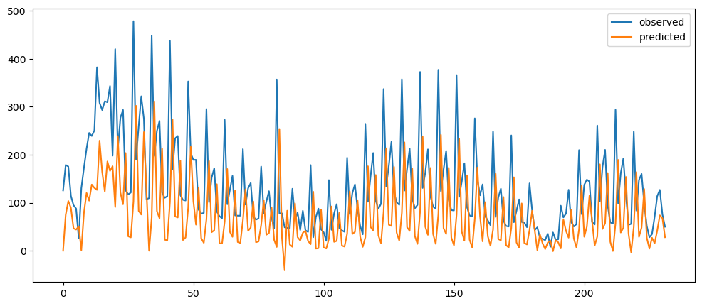
appendingTOR(tableOfResults, 'Ticket Sales', 'ARIMA - MA2', evaluateErrors(ticketSalesMA2Model))
tableOfResults| Unnamed: 0 | Data | Algorithm | MSE | RMSE | MAE |
|---|---|---|---|---|---|
| 1 | SP500 | Naive Forecasting | 0.315878 | 0.56203 | 0.325863 |
| 2 | FTSE | Naive Forecasting | 5.69646 | 2.38673 | 1.29783 |
| 3 | Gold | Naive Forecasting | 0.237289 | 0.487123 | 0.31245 |
| 4 | USDCUSDT Close Price | Naive Forecasting | 4.01536e-06 | 0.002004 | 0.001034 |
| 5 | USDCUSDT Tradecount | Naive Forecasting | 1.56376e+08 | 12505 | 7519.96 |
| 6 | Python Questions | Naive Forecasting | 1.00863e+06 | 1004.31 | 680.298 |
| 7 | Machine Learning Questions | Naive Forecasting | 3053.46 | 55.2581 | 35.4885 |
| 8 | Ticket Sales | Naive Forecasting | 12476 | 111.696 | 74.8537 |
| 9 | SP500 | Seasonal Forecasting - 60 | 24.0706 | 4.90618 | 3.19858 |
| 10 | SP500 | Seasonal Forecasting - 1440 | 578.648 | 24.0551 | 18.6964 |
| 11 | FTSE | Seasonal Forecasting - 60 | 358.944 | 18.9458 | 12.5549 |
| 12 | FTSE | Seasonal Forecasting - 1440 | 9305.27 | 96.4639 | 71.5358 |
| 13 | Gold | Seasonal Forecasting - 60 | 11.0817 | 3.32892 | 2.08104 |
| 14 | Gold | Seasonal Forecasting - 1440 | 297.39 | 17.245 | 12.2358 |
| 15 | USDCUSDT Close Price | Seasonal Forecasting | 1.41478e-05 | 0.003761 | 0.00176 |
| 16 | USDCUSDT Tradecount | Seasonal Forecasting | 2.76653e+08 | 16632.9 | 10558.5 |
| 17 | Python Questions | Seasonal Forecasting | 4.97505e+06 | 2230.48 | 1924.32 |
| 18 | Machine Learning Questions | Seasonal Forecasting | 14325.5 | 119.689 | 84.975 |
| 19 | Ticket Sales | Seasonal Forecasting | 3922.4 | 62.6291 | 37.0187 |
| 20 | SP500 | Average Forecasting - 60 | 8.21104 | 2.86549 | 1.84062 |
| 21 | SP500 | Average Forecasting - 1440 | 195.085 | 13.9673 | 10.6287 |
| 22 | FTSE | Average Forecasting - 60 | 122.369 | 11.0621 | 7.24807 |
| 23 | FTSE | Average Forecasting - 1440 | 3105.82 | 55.7299 | 40.9431 |
| 24 | Gold | Average Forecasting - 60 | 3.79681 | 1.94854 | 1.22559 |
| 25 | Gold | Average Forecasting - 1440 | 96.5074 | 9.82382 | 6.8452 |
| 26 | USDCUSDT Close Price | Average Forecasting | 6.51406e-06 | 0.002552 | 0.001187 |
| 27 | USDCUSDT Tradecount | Average Forecasting | 1.44419e+08 | 12017.5 | 7727.27 |
| 28 | Python Questions | Average Forecasting | 2.18019e+06 | 1476.55 | 1175.32 |
| 29 | Machine Learning Questions | Average Forecasting | 7140.3 | 84.5003 | 55.785 |
| 30 | Ticket Sales | Average Forecasting | 6061.2 | 77.8537 | 59.7301 |
| 31 | SP500 | Average Difference Forecasting - 60 | 0.322452 | 0.567849 | 0.332982 |
| 32 | SP500 | Average Difference Forecasting - 1440 | 0.316412 | 0.562505 | 0.326336 |
| 33 | FTSE | Average Difference Forecasting - 60 | 5.79875 | 2.40806 | 1.32178 |
| 34 | FTSE | Average Difference Forecasting - 1440 | 5.70723 | 2.38898 | 1.30033 |
| 35 | Gold | Average Difference Forecasting - 60 | 0.240423 | 0.49033 | 0.315994 |
| 36 | Gold | Average Difference Forecasting - 1440 | 0.237595 | 0.487437 | 0.313009 |
| 37 | USDCUSDT Close Price | Average Difference Forecasting | 4.53094e-06 | 0.002129 | 0.001103 |
| 38 | USDCUSDT Tradecount | Average Difference Forecasting | 1.64095e+08 | 12810 | 7724.69 |
| 39 | Python Questions | Average Difference Forecasting | 1.1445e+06 | 1069.81 | 751.801 |
| 40 | Machine Learning Questions | Average Difference Forecasting | 3399.79 | 58.3077 | 38.5563 |
| 41 | Ticket Sales | Average Difference Forecasting | 12936.3 | 113.738 | 76.6102 |
| 42 | SP500 | Naive Difference Forecasting | 0.553753 | 0.744146 | 0.456603 |
| 43 | FTSE | Naive Difference Forecasting | 10.796 | 3.28573 | 1.81081 |
| 44 | Gold | Naive Difference Forecasting | 0.521205 | 0.721946 | 0.480641 |
| 45 | USDCUSDT Close Price | Naive Difference Forecasting | 9.13676e-06 | 0.003023 | 0.001659 |
| 46 | USDCUSDT Tradecount | Naive Difference Forecasting | 4.15266e+08 | 20378.1 | 12089.8 |
| 47 | Python Questions | Naive Difference Forecasting | 2.34416e+06 | 1531.07 | 1117.71 |
| 48 | Machine Learning Questions | Naive Difference Forecasting | 6678.13 | 81.7198 | 51.9462 |
| 49 | Ticket Sales | Naive Difference Forecasting | 37594.4 | 193.893 | 136.398 |
| 50 | Gold | Autoregression | 0.167187 | 0.408885 | 0.270593 |
| 51 | SP500 | Autoregression | 0.181846 | 0.426434 | 0.236095 |
| 52 | Machine Learning Questions | Autoregression | 9493.88 | 97.4365 | 80.8513 |
| 53 | Ticket Sales | Autoregression | 12195.6 | 110.434 | 78.7188 |
| 54 | Gold | Manual ARIMA | 8.31094 | 2.88287 | 1.99452 |
| 55 | Ticket Sales | ARIMA - MA2 | 14257.6 | 119.405 | 93.6058 |
MA 3
ticketSalesMA3Model = exploringARIMA(ticketSalesData, 0, 0, 3)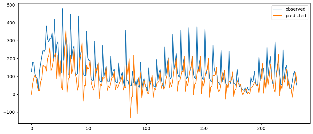
appendingTOR(tableOfResults, 'Ticket Sales', 'ARIMA - MA3', evaluateErrors(ticketSalesMA3Model))
tableOfResults| Unnamed: 0 | Data | Algorithm | MSE | RMSE | MAE |
|---|---|---|---|---|---|
| 1 | SP500 | Naive Forecasting | 0.315878 | 0.56203 | 0.325863 |
| 2 | FTSE | Naive Forecasting | 5.69646 | 2.38673 | 1.29783 |
| 3 | Gold | Naive Forecasting | 0.237289 | 0.487123 | 0.31245 |
| 4 | USDCUSDT Close Price | Naive Forecasting | 4.01536e-06 | 0.002004 | 0.001034 |
| 5 | USDCUSDT Tradecount | Naive Forecasting | 1.56376e+08 | 12505 | 7519.96 |
| 6 | Python Questions | Naive Forecasting | 1.00863e+06 | 1004.31 | 680.298 |
| 7 | Machine Learning Questions | Naive Forecasting | 3053.46 | 55.2581 | 35.4885 |
| 8 | Ticket Sales | Naive Forecasting | 12476 | 111.696 | 74.8537 |
| 9 | SP500 | Seasonal Forecasting - 60 | 24.0706 | 4.90618 | 3.19858 |
| 10 | SP500 | Seasonal Forecasting - 1440 | 578.648 | 24.0551 | 18.6964 |
| 11 | FTSE | Seasonal Forecasting - 60 | 358.944 | 18.9458 | 12.5549 |
| 12 | FTSE | Seasonal Forecasting - 1440 | 9305.27 | 96.4639 | 71.5358 |
| 13 | Gold | Seasonal Forecasting - 60 | 11.0817 | 3.32892 | 2.08104 |
| 14 | Gold | Seasonal Forecasting - 1440 | 297.39 | 17.245 | 12.2358 |
| 15 | USDCUSDT Close Price | Seasonal Forecasting | 1.41478e-05 | 0.003761 | 0.00176 |
| 16 | USDCUSDT Tradecount | Seasonal Forecasting | 2.76653e+08 | 16632.9 | 10558.5 |
| 17 | Python Questions | Seasonal Forecasting | 4.97505e+06 | 2230.48 | 1924.32 |
| 18 | Machine Learning Questions | Seasonal Forecasting | 14325.5 | 119.689 | 84.975 |
| 19 | Ticket Sales | Seasonal Forecasting | 3922.4 | 62.6291 | 37.0187 |
| 20 | SP500 | Average Forecasting - 60 | 8.21104 | 2.86549 | 1.84062 |
| 21 | SP500 | Average Forecasting - 1440 | 195.085 | 13.9673 | 10.6287 |
| 22 | FTSE | Average Forecasting - 60 | 122.369 | 11.0621 | 7.24807 |
| 23 | FTSE | Average Forecasting - 1440 | 3105.82 | 55.7299 | 40.9431 |
| 24 | Gold | Average Forecasting - 60 | 3.79681 | 1.94854 | 1.22559 |
| 25 | Gold | Average Forecasting - 1440 | 96.5074 | 9.82382 | 6.8452 |
| 26 | USDCUSDT Close Price | Average Forecasting | 6.51406e-06 | 0.002552 | 0.001187 |
| 27 | USDCUSDT Tradecount | Average Forecasting | 1.44419e+08 | 12017.5 | 7727.27 |
| 28 | Python Questions | Average Forecasting | 2.18019e+06 | 1476.55 | 1175.32 |
| 29 | Machine Learning Questions | Average Forecasting | 7140.3 | 84.5003 | 55.785 |
| 30 | Ticket Sales | Average Forecasting | 6061.2 | 77.8537 | 59.7301 |
| 31 | SP500 | Average Difference Forecasting - 60 | 0.322452 | 0.567849 | 0.332982 |
| 32 | SP500 | Average Difference Forecasting - 1440 | 0.316412 | 0.562505 | 0.326336 |
| 33 | FTSE | Average Difference Forecasting - 60 | 5.79875 | 2.40806 | 1.32178 |
| 34 | FTSE | Average Difference Forecasting - 1440 | 5.70723 | 2.38898 | 1.30033 |
| 35 | Gold | Average Difference Forecasting - 60 | 0.240423 | 0.49033 | 0.315994 |
| 36 | Gold | Average Difference Forecasting - 1440 | 0.237595 | 0.487437 | 0.313009 |
| 37 | USDCUSDT Close Price | Average Difference Forecasting | 4.53094e-06 | 0.002129 | 0.001103 |
| 38 | USDCUSDT Tradecount | Average Difference Forecasting | 1.64095e+08 | 12810 | 7724.69 |
| 39 | Python Questions | Average Difference Forecasting | 1.1445e+06 | 1069.81 | 751.801 |
| 40 | Machine Learning Questions | Average Difference Forecasting | 3399.79 | 58.3077 | 38.5563 |
| 41 | Ticket Sales | Average Difference Forecasting | 12936.3 | 113.738 | 76.6102 |
| 42 | SP500 | Naive Difference Forecasting | 0.553753 | 0.744146 | 0.456603 |
| 43 | FTSE | Naive Difference Forecasting | 10.796 | 3.28573 | 1.81081 |
| 44 | Gold | Naive Difference Forecasting | 0.521205 | 0.721946 | 0.480641 |
| 45 | USDCUSDT Close Price | Naive Difference Forecasting | 9.13676e-06 | 0.003023 | 0.001659 |
| 46 | USDCUSDT Tradecount | Naive Difference Forecasting | 4.15266e+08 | 20378.1 | 12089.8 |
| 47 | Python Questions | Naive Difference Forecasting | 2.34416e+06 | 1531.07 | 1117.71 |
| 48 | Machine Learning Questions | Naive Difference Forecasting | 6678.13 | 81.7198 | 51.9462 |
| 49 | Ticket Sales | Naive Difference Forecasting | 37594.4 | 193.893 | 136.398 |
| 50 | Gold | Autoregression | 0.167187 | 0.408885 | 0.270593 |
| 51 | SP500 | Autoregression | 0.181846 | 0.426434 | 0.236095 |
| 52 | Machine Learning Questions | Autoregression | 9493.88 | 97.4365 | 80.8513 |
| 53 | Ticket Sales | Autoregression | 12195.6 | 110.434 | 78.7188 |
| 54 | Gold | Manual ARIMA | 8.31094 | 2.88287 | 1.99452 |
| 55 | Ticket Sales | ARIMA - MA2 | 14257.6 | 119.405 | 93.6058 |
| 56 | Ticket Sales | ARIMA - MA3 | 9808.53 | 99.038 | 63.8928 |
MA 8 - 10
for i in range(8,11):
model = exploringARIMA(ticketSalesData, 0, 0, i)
appendingTOR(tableOfResults, 'Ticket Sales', 'ARIMA - MA' + str(i), evaluateErrors(model))
tableOfResults[tableOfResults['Data']=='Ticket Sales'].sort_values('MSE')
| Unnamed: 0 | Data | Algorithm | MSE | RMSE | MAE |
|---|---|---|---|---|---|
| 19 | Ticket Sales | Seasonal Forecasting | 3922.4 | 62.6291 | 37.0187 |
| 59 | Ticket Sales | ARIMA - MA10 | 5362.12 | 73.2265 | 49.4972 |
| 30 | Ticket Sales | Average Forecasting | 6061.2 | 77.8537 | 59.7301 |
| 58 | Ticket Sales | ARIMA - MA9 | 6219.51 | 78.8639 | 55.3295 |
| 57 | Ticket Sales | ARIMA - MA8 | 6453.79 | 80.3355 | 59.9724 |
| 56 | Ticket Sales | ARIMA - MA3 | 9808.53 | 99.038 | 63.8928 |
| 53 | Ticket Sales | Autoregression | 12195.6 | 110.434 | 78.7188 |
| 8 | Ticket Sales | Naive Forecasting | 12476 | 111.696 | 74.8537 |
| 41 | Ticket Sales | Average Difference Forecasting | 12936.3 | 113.738 | 76.6102 |
| 55 | Ticket Sales | ARIMA - MA2 | 14257.6 | 119.405 | 93.6058 |
| 49 | Ticket Sales | Naive Difference Forecasting | 37594.4 | 193.893 | 136.398 |
Visually we do not really see much improvement increasing the value of MA, however the results says otherwise. However it is still not the best. Let's try a higher number once again.
MA 20
ticketSalesMA20Model = exploringARIMA(ticketSalesData, 0, 0, 20)
appendingTOR(tableOfResults, 'Ticket Sales', 'ARIMA - MA20', evaluateErrors(ticketSalesMA20Model))
tableOfResults[tableOfResults['Data']=='Ticket Sales'].sort_values('MSE')
| Unnamed: 0 | Data | Algorithm | MSE | RMSE | MAE |
|---|---|---|---|---|---|
| 60 | Ticket Sales | ARIMA - MA20 | 3774.48 | 61.4368 | 42.521 |
| 19 | Ticket Sales | Seasonal Forecasting | 3922.4 | 62.6291 | 37.0187 |
| 59 | Ticket Sales | ARIMA - MA10 | 5362.12 | 73.2265 | 49.4972 |
| 30 | Ticket Sales | Average Forecasting | 6061.2 | 77.8537 | 59.7301 |
| 58 | Ticket Sales | ARIMA - MA9 | 6219.51 | 78.8639 | 55.3295 |
| 57 | Ticket Sales | ARIMA - MA8 | 6453.79 | 80.3355 | 59.9724 |
| 56 | Ticket Sales | ARIMA - MA3 | 9808.53 | 99.038 | 63.8928 |
| 53 | Ticket Sales | Autoregression | 12195.6 | 110.434 | 78.7188 |
| 8 | Ticket Sales | Naive Forecasting | 12476 | 111.696 | 74.8537 |
| 41 | Ticket Sales | Average Difference Forecasting | 12936.3 | 113.738 | 76.6102 |
| 55 | Ticket Sales | ARIMA - MA2 | 14257.6 | 119.405 | 93.6058 |
| 49 | Ticket Sales | Naive Difference Forecasting | 37594.4 | 193.893 | 136.398 |
As of the current observation, based on the ticket sales dataset, we can see that increase the MA lowers the errors.
Let's try only using I
for i in [1,2,5,10 ]:
model = exploringARIMA(ticketSalesData, 0, i, 0)
appendingTOR(tableOfResults, 'Ticket Sales', 'ARIMA - I' + str(i), evaluateErrors(model))
tableOfResults[tableOfResults['Data']=='Ticket Sales'].sort_values('MSE')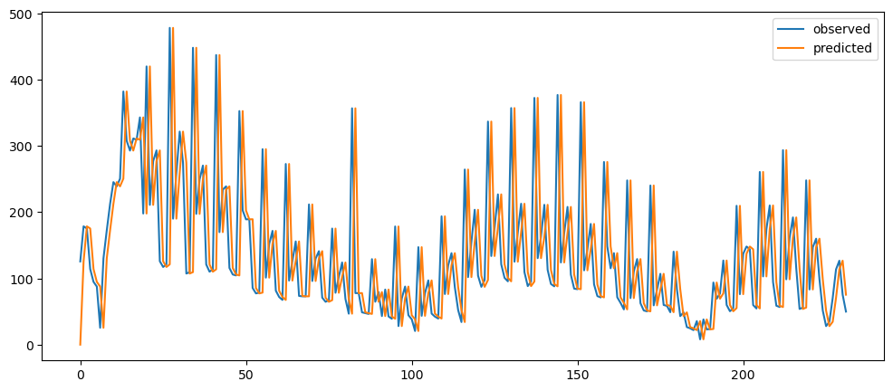
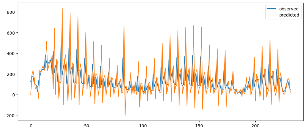
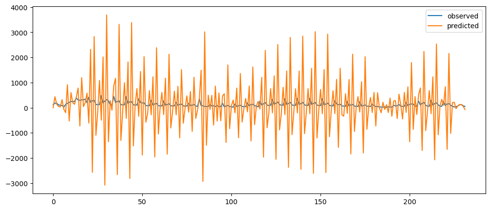
| Unnamed: 0 | Data | Algorithm | MSE | RMSE | MAE |
|---|---|---|---|---|---|
| 60 | Ticket Sales | ARIMA - MA20 | 3774.48 | 61.4368 | 42.521 |
| 19 | Ticket Sales | Seasonal Forecasting | 3922.4 | 62.6291 | 37.0187 |
| 59 | Ticket Sales | ARIMA - MA10 | 5362.11 | 73.2265 | 49.4972 |
| 30 | Ticket Sales | Average Forecasting | 6061.2 | 77.8537 | 59.7301 |
| 58 | Ticket Sales | ARIMA - MA9 | 6219.51 | 78.8639 | 55.3295 |
| 57 | Ticket Sales | ARIMA - MA8 | 6453.8 | 80.3355 | 59.9724 |
| 56 | Ticket Sales | ARIMA - MA3 | 9808.53 | 99.038 | 63.8928 |
| 53 | Ticket Sales | Autoregression | 12195.6 | 110.434 | 78.7188 |
| 8 | Ticket Sales | Naive Forecasting | 12476 | 111.696 | 74.8537 |
| 61 | Ticket Sales | ARIMA - I1 | 12490.3 | 111.76 | 75.0726 |
| 41 | Ticket Sales | Average Difference Forecasting | 12936.3 | 113.738 | 76.6102 |
| 55 | Ticket Sales | ARIMA - MA2 | 14257.6 | 119.405 | 93.6058 |
| 62 | Ticket Sales | ARIMA - I2 | 37338.9 | 193.233 | 135.811 |
| 49 | Ticket Sales | Naive Difference Forecasting | 37594.4 | 193.893 | 136.398 |
| 63 | Ticket Sales | ARIMA - I5 | 1.52389e+06 | 1234.46 | 926.465 |
| 64 | Ticket Sales | ARIMA - I10 | 1.08863e+09 | 32994.4 | 26180.1 |
As observed, I will need to be used sparingly as increase in I will quickly increase the predicted values.
I1 AM10
ticketSalesI1MA10Model = exploringARIMA(ticketSalesData, 0, 1, 10)
appendingTOR(tableOfResults, 'Ticket Sales', 'ARIMA - I1 MA10', evaluateErrors(ticketSalesI1MA10Model))
tableOfResults[tableOfResults['Data']=='Ticket Sales'].sort_values('MSE')
| Unnamed: 0 | Data | Algorithm | MSE | RMSE | MAE |
|---|---|---|---|---|---|
| 60 | Ticket Sales | ARIMA - MA20 | 3774.48 | 61.4368 | 42.521 |
| 19 | Ticket Sales | Seasonal Forecasting | 3922.4 | 62.6291 | 37.0187 |
| 65 | Ticket Sales | ARIMA - I1 MA10 | 4073.38 | 63.823 | 47.404 |
| 59 | Ticket Sales | ARIMA - MA10 | 5362.11 | 73.2265 | 49.4972 |
| 30 | Ticket Sales | Average Forecasting | 6061.2 | 77.8537 | 59.7301 |
| 58 | Ticket Sales | ARIMA - MA9 | 6219.51 | 78.8639 | 55.3295 |
| 57 | Ticket Sales | ARIMA - MA8 | 6453.8 | 80.3355 | 59.9724 |
| 56 | Ticket Sales | ARIMA - MA3 | 9808.53 | 99.038 | 63.8928 |
| 53 | Ticket Sales | Autoregression | 12195.6 | 110.434 | 78.7188 |
| 8 | Ticket Sales | Naive Forecasting | 12476 | 111.696 | 74.8537 |
| 61 | Ticket Sales | ARIMA - I1 | 12490.3 | 111.76 | 75.0726 |
| 41 | Ticket Sales | Average Difference Forecasting | 12936.3 | 113.738 | 76.6102 |
| 55 | Ticket Sales | ARIMA - MA2 | 14257.6 | 119.405 | 93.6058 |
| 62 | Ticket Sales | ARIMA - I2 | 37338.9 | 193.233 | 135.811 |
| 49 | Ticket Sales | Naive Difference Forecasting | 37594.4 | 193.893 | 136.398 |
| 63 | Ticket Sales | ARIMA - I5 | 1.52389e+06 | 1234.46 | 926.465 |
| 64 | Ticket Sales | ARIMA - I10 | 1.08863e+09 | 32994.4 | 26180.1 |
ticketSalesI1MA5Model = exploringARIMA(ticketSalesData, 0, 1, 5)
appendingTOR(tableOfResults, 'Ticket Sales', 'ARIMA - I1 MA5', evaluateErrors(ticketSalesI1MA5Model))
tableOfResults[tableOfResults['Data']=='Ticket Sales'].sort_values('MSE')
| Unnamed: 0 | Data | Algorithm | MSE | RMSE | MAE |
|---|---|---|---|---|---|
| 60 | Ticket Sales | ARIMA - MA20 | 3774.48 | 61.4368 | 42.521 |
| 19 | Ticket Sales | Seasonal Forecasting | 3922.4 | 62.6291 | 37.0187 |
| 65 | Ticket Sales | ARIMA - I1 MA10 | 4073.38 | 63.823 | 47.404 |
| 59 | Ticket Sales | ARIMA - MA10 | 5362.11 | 73.2265 | 49.4972 |
| 66 | Ticket Sales | ARIMA - I1 MA5 | 6030.57 | 77.6567 | 61.9688 |
| 30 | Ticket Sales | Average Forecasting | 6061.2 | 77.8537 | 59.7301 |
| 58 | Ticket Sales | ARIMA - MA9 | 6219.51 | 78.8639 | 55.3295 |
| 57 | Ticket Sales | ARIMA - MA8 | 6453.8 | 80.3355 | 59.9724 |
| 56 | Ticket Sales | ARIMA - MA3 | 9808.53 | 99.038 | 63.8928 |
| 53 | Ticket Sales | Autoregression | 12195.6 | 110.434 | 78.7188 |
| 8 | Ticket Sales | Naive Forecasting | 12476 | 111.696 | 74.8537 |
| 61 | Ticket Sales | ARIMA - I1 | 12490.3 | 111.76 | 75.0726 |
| 41 | Ticket Sales | Average Difference Forecasting | 12936.3 | 113.738 | 76.6102 |
| 55 | Ticket Sales | ARIMA - MA2 | 14257.6 | 119.405 | 93.6058 |
| 62 | Ticket Sales | ARIMA - I2 | 37338.9 | 193.233 | 135.811 |
| 49 | Ticket Sales | Naive Difference Forecasting | 37594.4 | 193.893 | 136.398 |
| 63 | Ticket Sales | ARIMA - I5 | 1.52389e+06 | 1234.46 | 926.465 |
| 64 | Ticket Sales | ARIMA - I10 | 1.08863e+09 | 32994.4 | 26180.1 |
ticketSalesI1MA5Model = exploringARIMA(ticketSalesData, 0, 1, 2)
appendingTOR(tableOfResults, 'Ticket Sales', 'ARIMA - I1 MA2', evaluateErrors(ticketSalesI1MA5Model))
tableOfResults[tableOfResults['Data']=='Ticket Sales'].sort_values('MSE')
| Unnamed: 0 | Data | Algorithm | MSE | RMSE | MAE |
|---|---|---|---|---|---|
| 60 | Ticket Sales | ARIMA - MA20 | 3774.48 | 61.4368 | 42.521 |
| 19 | Ticket Sales | Seasonal Forecasting | 3922.4 | 62.6291 | 37.0187 |
| 65 | Ticket Sales | ARIMA - I1 MA10 | 4073.38 | 63.823 | 47.404 |
| 59 | Ticket Sales | ARIMA - MA10 | 5362.11 | 73.2265 | 49.4972 |
| 66 | Ticket Sales | ARIMA - I1 MA5 | 6030.57 | 77.6567 | 61.9688 |
| 30 | Ticket Sales | Average Forecasting | 6061.2 | 77.8537 | 59.7301 |
| 58 | Ticket Sales | ARIMA - MA9 | 6219.51 | 78.8639 | 55.3295 |
| 57 | Ticket Sales | ARIMA - MA8 | 6453.8 | 80.3355 | 59.9724 |
| 67 | Ticket Sales | ARIMA - I1 MA2 | 6726.3 | 82.014 | 62.7677 |
| 56 | Ticket Sales | ARIMA - MA3 | 9808.53 | 99.038 | 63.8928 |
| 53 | Ticket Sales | Autoregression | 12195.6 | 110.434 | 78.7188 |
| 8 | Ticket Sales | Naive Forecasting | 12476 | 111.696 | 74.8537 |
| 61 | Ticket Sales | ARIMA - I1 | 12490.3 | 111.76 | 75.0726 |
| 41 | Ticket Sales | Average Difference Forecasting | 12936.3 | 113.738 | 76.6102 |
| 55 | Ticket Sales | ARIMA - MA2 | 14257.6 | 119.405 | 93.6058 |
| 62 | Ticket Sales | ARIMA - I2 | 37338.9 | 193.233 | 135.811 |
| 49 | Ticket Sales | Naive Difference Forecasting | 37594.4 | 193.893 | 136.398 |
| 63 | Ticket Sales | ARIMA - I5 | 1.52389e+06 | 1234.46 | 926.465 |
| 64 | Ticket Sales | ARIMA - I10 | 1.08863e+09 | 32994.4 | 26180.1 |
ticketSalesI2MA10Model = exploringARIMA(ticketSalesData, 0, 2, 10)
appendingTOR(tableOfResults, 'Ticket Sales', 'ARIMA - I2 MA10', evaluateErrors(ticketSalesI2MA10Model))
tableOfResults[tableOfResults['Data']=='Ticket Sales'].sort_values('MSE')
| Unnamed: 0 | Data | Algorithm | MSE | RMSE | MAE |
|---|---|---|---|---|---|
| 60 | Ticket Sales | ARIMA - MA20 | 3774.48 | 61.4368 | 42.521 |
| 19 | Ticket Sales | Seasonal Forecasting | 3922.4 | 62.6291 | 37.0187 |
| 65 | Ticket Sales | ARIMA - I1 MA10 | 4073.38 | 63.823 | 47.404 |
| 68 | Ticket Sales | ARIMA - I2 MA10 | 5306.96 | 72.8489 | 54.751 |
| 59 | Ticket Sales | ARIMA - MA10 | 5362.11 | 73.2265 | 49.4972 |
| 66 | Ticket Sales | ARIMA - I1 MA5 | 6030.57 | 77.6567 | 61.9688 |
| 30 | Ticket Sales | Average Forecasting | 6061.2 | 77.8537 | 59.7301 |
| 58 | Ticket Sales | ARIMA - MA9 | 6219.51 | 78.8639 | 55.3295 |
| 57 | Ticket Sales | ARIMA - MA8 | 6453.8 | 80.3355 | 59.9724 |
| 67 | Ticket Sales | ARIMA - I1 MA2 | 6726.3 | 82.014 | 62.7677 |
| 56 | Ticket Sales | ARIMA - MA3 | 9808.53 | 99.038 | 63.8928 |
| 53 | Ticket Sales | Autoregression | 12195.6 | 110.434 | 78.7188 |
| 8 | Ticket Sales | Naive Forecasting | 12476 | 111.696 | 74.8537 |
| 61 | Ticket Sales | ARIMA - I1 | 12490.3 | 111.76 | 75.0726 |
| 41 | Ticket Sales | Average Difference Forecasting | 12936.3 | 113.738 | 76.6102 |
| 55 | Ticket Sales | ARIMA - MA2 | 14257.6 | 119.405 | 93.6058 |
| 62 | Ticket Sales | ARIMA - I2 | 37338.9 | 193.233 | 135.811 |
| 49 | Ticket Sales | Naive Difference Forecasting | 37594.4 | 193.893 | 136.398 |
| 63 | Ticket Sales | ARIMA - I5 | 1.52389e+06 | 1234.46 | 926.465 |
| 64 | Ticket Sales | ARIMA - I10 | 1.08863e+09 | 32994.4 | 26180.1 |
As of the current observations, MA20 is still the highest at the moment. However, using higher value MA with I value of 1, is performing well
Now let's explore ARIMA.
A7 I1 MA2,3,5,10
for i in [2,3,5,10]:
model = exploringARIMA(ticketSalesData, 7, 1, i)
appendingTOR(tableOfResults, 'Ticket Sales', 'ARIMA - A7 I1 MA' + str(i), evaluateErrors(model))
tableOfResults[tableOfResults['Data']=='Ticket Sales'].sort_values('MSE')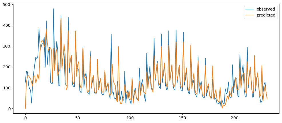
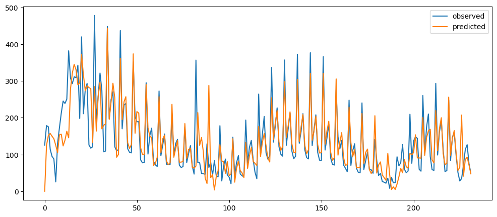

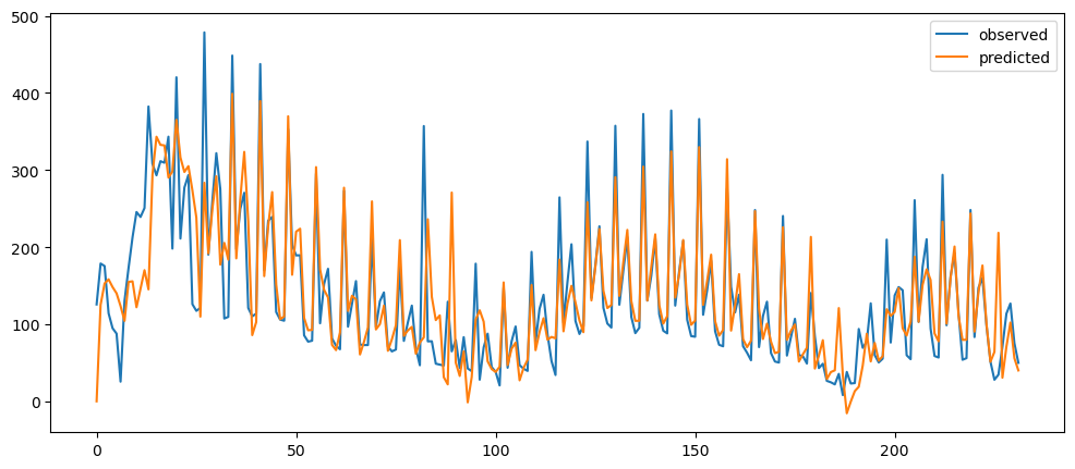
| Unnamed: 0 | Data | Algorithm | MSE | RMSE | MAE |
|---|---|---|---|---|---|
| 72 | Ticket Sales | ARIMA - A7 I1 MA10 | 2805.43 | 52.9663 | 34.2589 |
| 71 | Ticket Sales | ARIMA - A7 I1 MA5 | 2835.07 | 53.2454 | 33.3404 |
| 70 | Ticket Sales | ARIMA - A7 I1 MA3 | 2875.15 | 53.6205 | 33.8151 |
| 69 | Ticket Sales | ARIMA - A7 I1 MA2 | 2900.55 | 53.8568 | 33.7684 |
| 60 | Ticket Sales | ARIMA - MA20 | 3774.48 | 61.4368 | 42.521 |
| 19 | Ticket Sales | Seasonal Forecasting | 3922.4 | 62.6291 | 37.0187 |
| 65 | Ticket Sales | ARIMA - I1 MA10 | 4073.38 | 63.823 | 47.404 |
| 68 | Ticket Sales | ARIMA - I2 MA10 | 5306.96 | 72.8489 | 54.751 |
| 59 | Ticket Sales | ARIMA - MA10 | 5362.11 | 73.2265 | 49.4972 |
| 66 | Ticket Sales | ARIMA - I1 MA5 | 6030.57 | 77.6567 | 61.9688 |
| 30 | Ticket Sales | Average Forecasting | 6061.2 | 77.8537 | 59.7301 |
| 58 | Ticket Sales | ARIMA - MA9 | 6219.51 | 78.8639 | 55.3295 |
| 57 | Ticket Sales | ARIMA - MA8 | 6453.8 | 80.3355 | 59.9724 |
| 67 | Ticket Sales | ARIMA - I1 MA2 | 6726.3 | 82.014 | 62.7677 |
| 56 | Ticket Sales | ARIMA - MA3 | 9808.53 | 99.038 | 63.8928 |
| 53 | Ticket Sales | Autoregression | 12195.6 | 110.434 | 78.7188 |
| 8 | Ticket Sales | Naive Forecasting | 12476 | 111.696 | 74.8537 |
| 61 | Ticket Sales | ARIMA - I1 | 12490.3 | 111.76 | 75.0726 |
| 41 | Ticket Sales | Average Difference Forecasting | 12936.3 | 113.738 | 76.6102 |
| 55 | Ticket Sales | ARIMA - MA2 | 14257.6 | 119.405 | 93.6058 |
| 62 | Ticket Sales | ARIMA - I2 | 37338.9 | 193.233 | 135.811 |
| 49 | Ticket Sales | Naive Difference Forecasting | 37594.4 | 193.893 | 136.398 |
| 63 | Ticket Sales | ARIMA - I5 | 1.52389e+06 | 1234.46 | 926.465 |
| 64 | Ticket Sales | ARIMA - I10 | 1.08863e+09 | 32994.4 | 26180.1 |
When using Autoregression, Intergrated and Moving Average, all together, it performed the best, according the RMSE, MSE and MAE. We now will try a few iterations and parameters with the gold data.
Gold Data
arimaGoldData = goldData.reset_index()['Close'][:30000]
arimaGoldData.plot()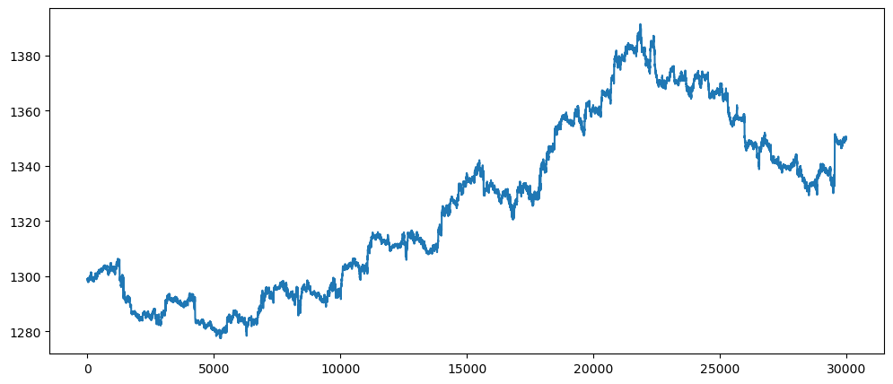
MA Test
for i in [1,2,5,10]:
model = exploringARIMA(arimaGoldData, 0,0,i)
appendingTOR(tableOfResults, 'Gold', 'ARIMA - MA' + str(i), evaluateErrors(model))
tableOfResults[tableOfResults['Data'] == 'Gold'].sort_values('MSE')| Unnamed: 0 | Data | Algorithm | MSE | RMSE | MAE |
|---|---|---|---|---|---|
| 50 | Gold | Autoregression | 0.167187 | 0.408885 | 0.270593 |
| 3 | Gold | Naive Forecasting | 0.237289 | 0.487123 | 0.31245 |
| 36 | Gold | Average Difference Forecasting - 1440 | 0.237595 | 0.487437 | 0.313009 |
| 35 | Gold | Average Difference Forecasting - 60 | 0.240423 | 0.49033 | 0.315994 |
| 44 | Gold | Naive Difference Forecasting | 0.521205 | 0.721946 | 0.480641 |
| 24 | Gold | Average Forecasting - 60 | 3.79681 | 1.94854 | 1.22559 |
| 54 | Gold | Manual ARIMA | 8.31094 | 2.88287 | 1.99452 |
| 13 | Gold | Seasonal Forecasting - 60 | 11.0817 | 3.32892 | 2.08104 |
| 25 | Gold | Average Forecasting - 1440 | 96.5074 | 9.82382 | 6.8452 |
| 14 | Gold | Seasonal Forecasting - 1440 | 297.39 | 17.245 | 12.2358 |
| 75 | Gold | ARIMA - MA5 | 155277 | 394.052 | 316.199 |
| 74 | Gold | ARIMA - MA2 | 194643 | 441.184 | 368.211 |
| 73 | Gold | ARIMA - MA1 | 439874 | 663.23 | 662.926 |
| 76 | Gold | ARIMA - MA10 | 1.51433e+20 | 1.23058e+10 | 1.21355e+10 |
As shown above, using only the MA alone does not seem to be performing good, and actually the worst ones when compared to the other models here, especially when there is no pre-processing done. By having I, the differencing performed, the performance should improve
I Test
for i in [1,2,5,10]:
model = exploringARIMA(arimaGoldData, 0,i,0)
appendingTOR(tableOfResults, 'Gold', 'ARIMA - I' + str(i), evaluateErrors(model))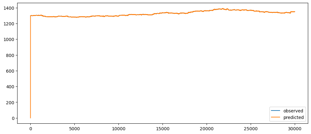
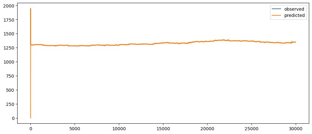
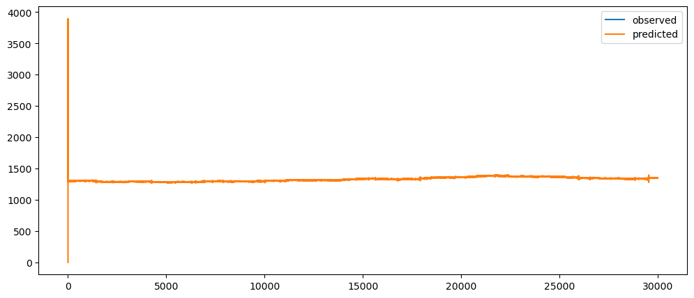
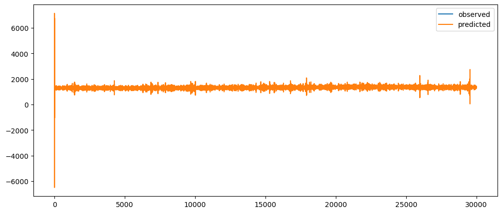
tableOfResults[tableOfResults['Data'] == 'Gold'].sort_values('MSE')| Unnamed: 0 | Data | Algorithm | MSE | RMSE | MAE |
|---|---|---|---|---|---|
| 50 | Gold | Autoregression | 0.167187 | 0.408885 | 0.270593 |
| 3 | Gold | Naive Forecasting | 0.237289 | 0.487123 | 0.31245 |
| 36 | Gold | Average Difference Forecasting - 1440 | 0.237595 | 0.487437 | 0.313009 |
| 35 | Gold | Average Difference Forecasting - 60 | 0.240423 | 0.49033 | 0.315994 |
| 44 | Gold | Naive Difference Forecasting | 0.521205 | 0.721946 | 0.480641 |
| 24 | Gold | Average Forecasting - 60 | 3.79681 | 1.94854 | 1.22559 |
| 54 | Gold | Manual ARIMA | 8.31094 | 2.88287 | 1.99452 |
| 13 | Gold | Seasonal Forecasting - 60 | 11.0817 | 3.32892 | 2.08104 |
| 77 | Gold | ARIMA - I1 | 56.3362 | 7.50575 | 0.295501 |
| 78 | Gold | ARIMA - I2 | 70.5507 | 8.39945 | 0.459694 |
| 25 | Gold | Average Forecasting - 1440 | 96.5074 | 9.82382 | 6.8452 |
| 14 | Gold | Seasonal Forecasting - 1440 | 297.39 | 17.245 | 12.2358 |
| 79 | Gold | ARIMA - I5 | 350.547 | 18.7229 | 2.61938 |
| 80 | Gold | ARIMA - I10 | 12166.7 | 110.303 | 66.0953 |
| 75 | Gold | ARIMA - MA5 | 155277 | 394.052 | 316.199 |
| 74 | Gold | ARIMA - MA2 | 194643 | 441.184 | 368.211 |
| 73 | Gold | ARIMA - MA1 | 439874 | 663.23 | 662.926 |
| 76 | Gold | ARIMA - MA10 | 1.51433e+20 | 1.23058e+10 | 1.21355e+10 |
The I of 1, is the best performing one so far.
Let's try having the I set to 1, and we will see if MA 1 2 or 5 will perform better.
I1 MA Test
for i in [1,2,5]:
model = exploringARIMA(arimaGoldData, 0,1,i)
appendingTOR(tableOfResults, 'Gold', 'ARIMA - I1 MA' + str(i), evaluateErrors(model))


tableOfResults[tableOfResults['Data'] == 'Gold'].sort_values('MSE')| Unnamed: 0 | Data | Algorithm | MSE | RMSE | MAE |
|---|---|---|---|---|---|
| 50 | Gold | Autoregression | 0.167187 | 0.408885 | 0.270593 |
| 3 | Gold | Naive Forecasting | 0.237289 | 0.487123 | 0.31245 |
| 36 | Gold | Average Difference Forecasting - 1440 | 0.237595 | 0.487437 | 0.313009 |
| 35 | Gold | Average Difference Forecasting - 60 | 0.240423 | 0.49033 | 0.315994 |
| 44 | Gold | Naive Difference Forecasting | 0.521205 | 0.721946 | 0.480641 |
| 24 | Gold | Average Forecasting - 60 | 3.79681 | 1.94854 | 1.22559 |
| 54 | Gold | Manual ARIMA | 8.31094 | 2.88287 | 1.99452 |
| 13 | Gold | Seasonal Forecasting - 60 | 11.0817 | 3.32892 | 2.08104 |
| 83 | Gold | ARIMA - I1 MA5 | 56.3336 | 7.50557 | 0.29298 |
| 82 | Gold | ARIMA - I1 MA2 | 56.3336 | 7.50557 | 0.292994 |
| 81 | Gold | ARIMA - I1 MA1 | 56.3337 | 7.50558 | 0.293011 |
| 77 | Gold | ARIMA - I1 | 56.3362 | 7.50575 | 0.295501 |
| 78 | Gold | ARIMA - I2 | 70.5507 | 8.39945 | 0.459694 |
| 25 | Gold | Average Forecasting - 1440 | 96.5074 | 9.82382 | 6.8452 |
| 14 | Gold | Seasonal Forecasting - 1440 | 297.39 | 17.245 | 12.2358 |
| 79 | Gold | ARIMA - I5 | 350.547 | 18.7229 | 2.61938 |
| 80 | Gold | ARIMA - I10 | 12166.7 | 110.303 | 66.0953 |
| 75 | Gold | ARIMA - MA5 | 155277 | 394.052 | 316.199 |
| 74 | Gold | ARIMA - MA2 | 194643 | 441.184 | 368.211 |
| 73 | Gold | ARIMA - MA1 | 439874 | 663.23 | 662.926 |
| 76 | Gold | ARIMA - MA10 | 1.51433e+20 | 1.23058e+10 | 1.21355e+10 |
It seems that MA 5 is the better performing one by only a very small margin. Next we explore implementing the autoregression
AR I1 MA5 Test
plot_pacf(arimaGoldData)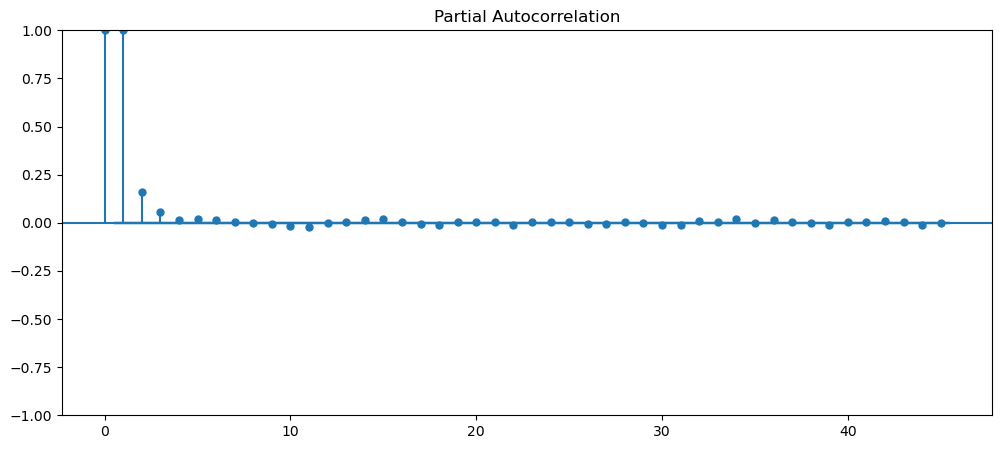

Based on the PACF test, we can see that up to an AR 4 should be good. However, we can also increase it to see how it performs
for i in [4, 8, 15, 20]:
model = exploringARIMA(arimaGoldData, i,1,5)
appendingTOR(tableOfResults, 'Gold', 'ARIMA - A' + str(i) + ' I1 MA5', evaluateErrors(model))


tableOfResults[tableOfResults['Data'] == 'Gold'].sort_values('MSE')| Unnamed: 0 | Data | Algorithm | MSE | RMSE | MAE |
|---|---|---|---|---|---|
| 50 | Gold | Autoregression | 0.167187 | 0.408885 | 0.270593 |
| 3 | Gold | Naive Forecasting | 0.237289 | 0.487123 | 0.31245 |
| 36 | Gold | Average Difference Forecasting - 1440 | 0.237595 | 0.487437 | 0.313009 |
| 35 | Gold | Average Difference Forecasting - 60 | 0.240423 | 0.49033 | 0.315994 |
| 44 | Gold | Naive Difference Forecasting | 0.521205 | 0.721946 | 0.480641 |
| 24 | Gold | Average Forecasting - 60 | 3.79681 | 1.94854 | 1.22559 |
| 54 | Gold | Manual ARIMA | 8.31094 | 2.88287 | 1.99452 |
| 13 | Gold | Seasonal Forecasting - 60 | 11.0817 | 3.32892 | 2.08104 |
| 87 | Gold | ARIMA - A20 I1 MA5 | 56.3334 | 7.50556 | 0.293046 |
| 86 | Gold | ARIMA - A15 I1 MA5 | 56.3334 | 7.50556 | 0.293048 |
| 85 | Gold | ARIMA - A8 I1 MA5 | 56.3334 | 7.50556 | 0.293065 |
| 84 | Gold | ARIMA - A4 I1 MA5 | 56.3335 | 7.50556 | 0.293029 |
| 83 | Gold | ARIMA - I1 MA5 | 56.3336 | 7.50557 | 0.29298 |
| 82 | Gold | ARIMA - I1 MA2 | 56.3336 | 7.50557 | 0.292994 |
| 81 | Gold | ARIMA - I1 MA1 | 56.3337 | 7.50558 | 0.293011 |
| 77 | Gold | ARIMA - I1 | 56.3362 | 7.50575 | 0.295501 |
| 78 | Gold | ARIMA - I2 | 70.5507 | 8.39945 | 0.459694 |
| 25 | Gold | Average Forecasting - 1440 | 96.5074 | 9.82382 | 6.8452 |
| 14 | Gold | Seasonal Forecasting - 1440 | 297.39 | 17.245 | 12.2358 |
| 79 | Gold | ARIMA - I5 | 350.547 | 18.7229 | 2.61938 |
| 80 | Gold | ARIMA - I10 | 12166.7 | 110.303 | 66.0953 |
| 75 | Gold | ARIMA - MA5 | 155277 | 394.052 | 316.199 |
| 74 | Gold | ARIMA - MA2 | 194643 | 441.184 | 368.211 |
| 73 | Gold | ARIMA - MA1 | 439874 | 663.23 | 662.926 |
| 76 | Gold | ARIMA - MA10 | 1.51433e+20 | 1.23058e+10 | 1.21355e+10 |
While it is the best performing ones so far, it still does beat the earlier simple algorithms that were used.
Autoreg only
autoregGold4 = exploringARIMA(arimaGoldData, 4, 0, 0)
autoregGold4[1:].plot()
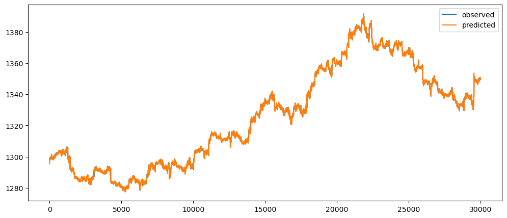
appendingTOR(tableOfResults, 'Gold', 'ARIMA - A4', evaluateErrors(autoregGold4))
tableOfResults[tableOfResults['Data'] == 'Gold'].sort_values('MSE')| Unnamed: 0 | Data | Algorithm | MSE | RMSE | MAE |
|---|---|---|---|---|---|
| 50 | Gold | Autoregression | 0.167187 | 0.408885 | 0.270593 |
| 3 | Gold | Naive Forecasting | 0.237289 | 0.487123 | 0.31245 |
| 36 | Gold | Average Difference Forecasting - 1440 | 0.237595 | 0.487437 | 0.313009 |
| 35 | Gold | Average Difference Forecasting - 60 | 0.240423 | 0.49033 | 0.315994 |
| 44 | Gold | Naive Difference Forecasting | 0.521205 | 0.721946 | 0.480641 |
| 24 | Gold | Average Forecasting - 60 | 3.79681 | 1.94854 | 1.22559 |
| 54 | Gold | Manual ARIMA | 8.31094 | 2.88287 | 1.99452 |
| 13 | Gold | Seasonal Forecasting - 60 | 11.0817 | 3.32892 | 2.08104 |
| 87 | Gold | ARIMA - A20 I1 MA5 | 56.3334 | 7.50556 | 0.293046 |
| 86 | Gold | ARIMA - A15 I1 MA5 | 56.3334 | 7.50556 | 0.293048 |
| 85 | Gold | ARIMA - A8 I1 MA5 | 56.3334 | 7.50556 | 0.293065 |
| 84 | Gold | ARIMA - A4 I1 MA5 | 56.3335 | 7.50556 | 0.293029 |
| 83 | Gold | ARIMA - I1 MA5 | 56.3336 | 7.50557 | 0.29298 |
| 82 | Gold | ARIMA - I1 MA2 | 56.3336 | 7.50557 | 0.292994 |
| 81 | Gold | ARIMA - I1 MA1 | 56.3337 | 7.50558 | 0.293011 |
| 77 | Gold | ARIMA - I1 | 56.3362 | 7.50575 | 0.295501 |
| 88 | Gold | ARIMA - A4 | 56.3762 | 7.50841 | 0.334332 |
| 78 | Gold | ARIMA - I2 | 70.5507 | 8.39945 | 0.459694 |
| 25 | Gold | Average Forecasting - 1440 | 96.5074 | 9.82382 | 6.8452 |
| 14 | Gold | Seasonal Forecasting - 1440 | 297.39 | 17.245 | 12.2358 |
| 79 | Gold | ARIMA - I5 | 350.547 | 18.7229 | 2.61938 |
| 80 | Gold | ARIMA - I10 | 12166.7 | 110.303 | 66.0953 |
| 75 | Gold | ARIMA - MA5 | 155277 | 394.052 | 316.199 |
| 74 | Gold | ARIMA - MA2 | 194643 | 441.184 | 368.211 |
| 73 | Gold | ARIMA - MA1 | 439874 | 663.23 | 662.926 |
| 76 | Gold | ARIMA - MA10 | 1.51433e+20 | 1.23058e+10 | 1.21355e+10 |
We would think that the autoregression 4 model would perform good, however, it did not and it is the middle of the pack
tableOfResults[tableOfResults['Data'] == 'Ticket Sales'].sort_values('MSE')| Unnamed: 0 | Data | Algorithm | MSE | RMSE | MAE |
|---|---|---|---|---|---|
| 72 | Ticket Sales | ARIMA - A7 I1 MA10 | 2805.43 | 52.9663 | 34.2589 |
| 71 | Ticket Sales | ARIMA - A7 I1 MA5 | 2835.07 | 53.2454 | 33.3404 |
| 70 | Ticket Sales | ARIMA - A7 I1 MA3 | 2875.15 | 53.6205 | 33.8151 |
| 69 | Ticket Sales | ARIMA - A7 I1 MA2 | 2900.55 | 53.8568 | 33.7684 |
| 60 | Ticket Sales | ARIMA - MA20 | 3774.48 | 61.4368 | 42.521 |
| 19 | Ticket Sales | Seasonal Forecasting | 3922.4 | 62.6291 | 37.0187 |
| 65 | Ticket Sales | ARIMA - I1 MA10 | 4073.38 | 63.823 | 47.404 |
| 68 | Ticket Sales | ARIMA - I2 MA10 | 5306.96 | 72.8489 | 54.751 |
| 59 | Ticket Sales | ARIMA - MA10 | 5362.11 | 73.2265 | 49.4972 |
| 66 | Ticket Sales | ARIMA - I1 MA5 | 6030.57 | 77.6567 | 61.9688 |
| 30 | Ticket Sales | Average Forecasting | 6061.2 | 77.8537 | 59.7301 |
| 58 | Ticket Sales | ARIMA - MA9 | 6219.51 | 78.8639 | 55.3295 |
| 57 | Ticket Sales | ARIMA - MA8 | 6453.8 | 80.3355 | 59.9724 |
| 67 | Ticket Sales | ARIMA - I1 MA2 | 6726.3 | 82.014 | 62.7677 |
| 56 | Ticket Sales | ARIMA - MA3 | 9808.53 | 99.038 | 63.8928 |
| 53 | Ticket Sales | Autoregression | 12195.6 | 110.434 | 78.7188 |
| 8 | Ticket Sales | Naive Forecasting | 12476 | 111.696 | 74.8537 |
| 61 | Ticket Sales | ARIMA - I1 | 12490.3 | 111.76 | 75.0726 |
| 41 | Ticket Sales | Average Difference Forecasting | 12936.3 | 113.738 | 76.6102 |
| 55 | Ticket Sales | ARIMA - MA2 | 14257.6 | 119.405 | 93.6058 |
| 62 | Ticket Sales | ARIMA - I2 | 37338.9 | 193.233 | 135.811 |
| 49 | Ticket Sales | Naive Difference Forecasting | 37594.4 | 193.893 | 136.398 |
| 63 | Ticket Sales | ARIMA - I5 | 1.52389e+06 | 1234.46 | 926.465 |
| 64 | Ticket Sales | ARIMA - I10 | 1.08863e+09 | 32994.4 | 26180.1 |
Seasonal ARIMA
We will again trying SARIMA with and the tickets sales
ticketSalesData.plot()
sm.tsa.arima.ARIMA(ticketSalesData, order=(5,1,5), seasonal_order=(7,1,5,7), trend = 'n').fit().predict().plot()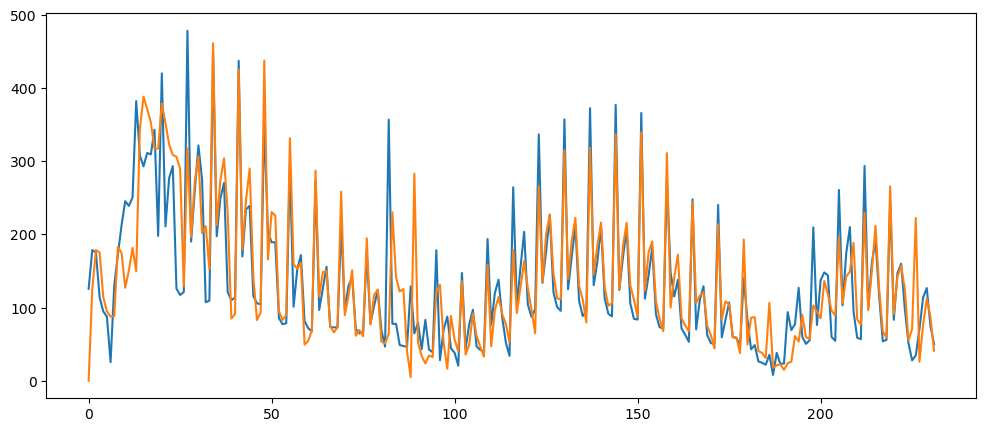
As shown, we can add more parameters given to the function. We can add a seasonal component to in, as shown in the seasonal_order. the first three supposed to be representing the same 3 values as the ones in order, and then the last value supposed to be representing the seasonality expectation. If we expect the seasons to be weekly, we can use 7, assume each row is one day, like this case. Seeing this site explains that the order was for trend, and seasonal order is to address the seasonality.
However, there are just too many parameters. Therefore, we will just be running loops and appending the results into the table. But we will be keeping the order parameters
def exploringSARIMA(data, p, q, r, m):
model = sm.tsa.arima.ARIMA(ticketSalesData, order=(5,1,5), seasonal_order=(p,q,r,m), trend = 'n').fit()
results = pd.DataFrame(data.rename('observed'))
results['predicted'] = model.predict()
results.plot()
return resultsfor p in range(5, 10):
for r in range(3,7):
model = exploringSARIMA(ticketSalesData, p, 1, r, 7)
appendingTOR(tableOfResults, 'Ticket Sales', 'SARIMA - p' +
str(p) + ' q' + str(1) + ' r' + str(r) + ' m' + str(7),
evaluateErrors(model)
)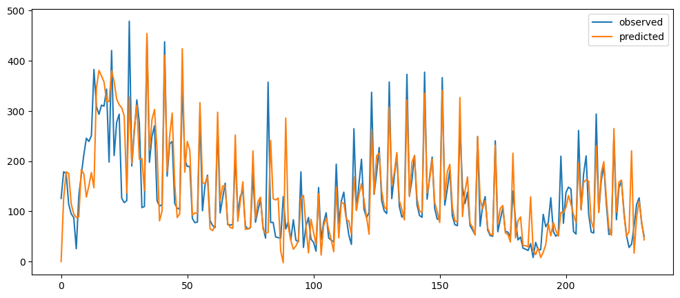

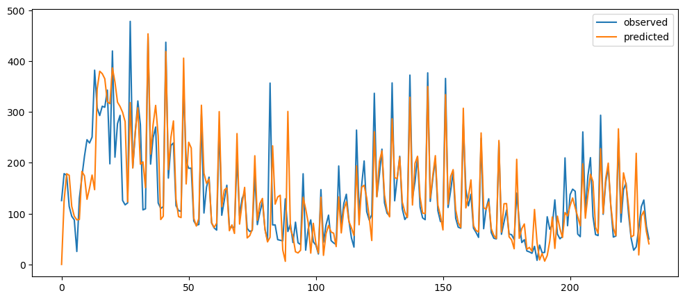

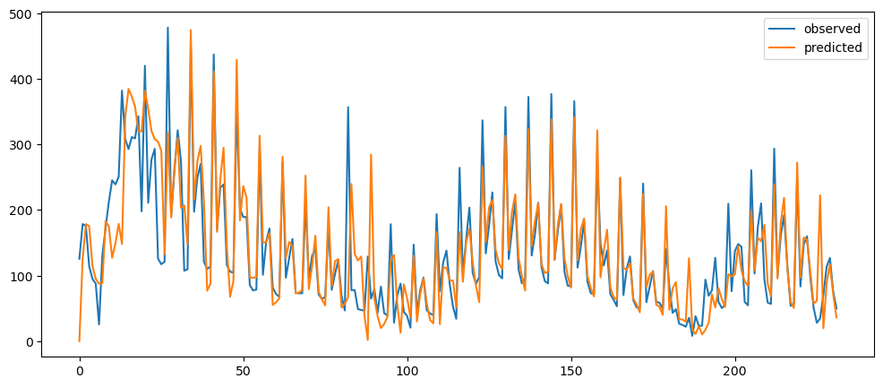


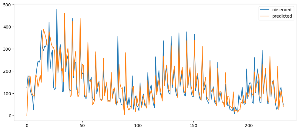
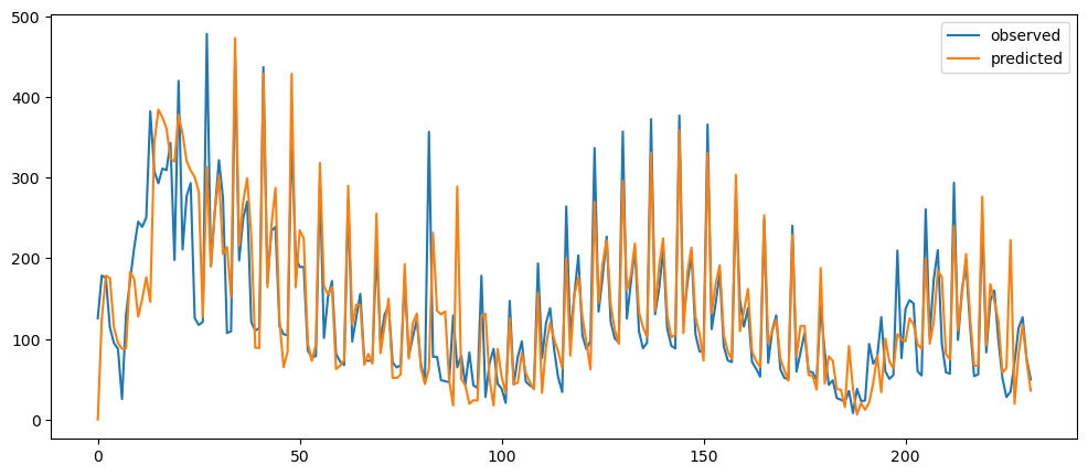

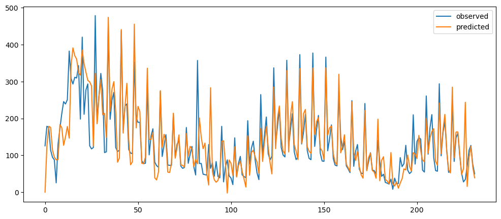


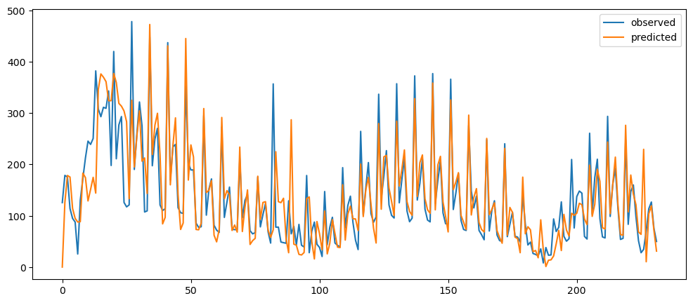
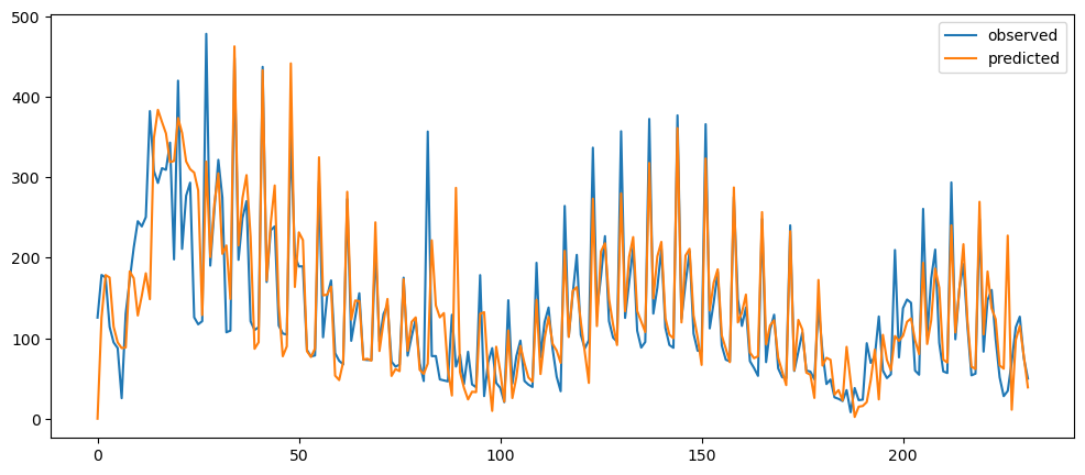
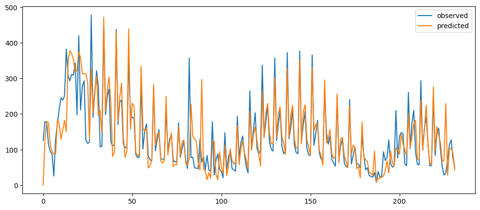
tableOfResults[tableOfResults['Data'] == 'Ticket Sales'].sort_values('MSE')| Unnamed: 0 | Data | Algorithm | MSE | RMSE | MAE |
|---|---|---|---|---|---|
| 72 | Ticket Sales | ARIMA - A7 I1 MA10 | 2805.43 | 52.9663 | 34.2589 |
| 71 | Ticket Sales | ARIMA - A7 I1 MA5 | 2835.07 | 53.2454 | 33.3404 |
| 70 | Ticket Sales | ARIMA - A7 I1 MA3 | 2875.15 | 53.6205 | 33.8151 |
| 108 | Ticket Sales | SARIMA - p9 q1 r6 m7 | 2882.86 | 53.6923 | 33.7857 |
| 105 | Ticket Sales | SARIMA - p9 q1 r3 m7 | 2884.03 | 53.7032 | 34.02 |
| 106 | Ticket Sales | SARIMA - p9 q1 r4 m7 | 2890.3 | 53.7616 | 34.1163 |
| 107 | Ticket Sales | SARIMA - p9 q1 r5 m7 | 2895.94 | 53.814 | 33.693 |
| 103 | Ticket Sales | SARIMA - p8 q1 r5 m7 | 2900.32 | 53.8546 | 33.5066 |
| 69 | Ticket Sales | ARIMA - A7 I1 MA2 | 2900.55 | 53.8568 | 33.7684 |
| 102 | Ticket Sales | SARIMA - p8 q1 r4 m7 | 2907.21 | 53.9185 | 34.1786 |
| 100 | Ticket Sales | SARIMA - p7 q1 r6 m7 | 2920.49 | 54.0415 | 33.954 |
| 101 | Ticket Sales | SARIMA - p8 q1 r3 m7 | 2935.23 | 54.1777 | 34.1753 |
| 97 | Ticket Sales | SARIMA - p7 q1 r3 m7 | 2940.85 | 54.2296 | 33.917 |
| 104 | Ticket Sales | SARIMA - p8 q1 r6 m7 | 2941.32 | 54.234 | 34.4356 |
| 93 | Ticket Sales | SARIMA - p6 q1 r3 m7 | 2947.68 | 54.2926 | 33.6726 |
| 96 | Ticket Sales | SARIMA - p6 q1 r6 m7 | 2948.95 | 54.3043 | 33.8336 |
| 98 | Ticket Sales | SARIMA - p7 q1 r4 m7 | 2952.75 | 54.3392 | 33.7096 |
| 99 | Ticket Sales | SARIMA - p7 q1 r5 m7 | 2953.18 | 54.3432 | 34.2208 |
| 95 | Ticket Sales | SARIMA - p6 q1 r5 m7 | 2958.34 | 54.3906 | 34.2589 |
| 90 | Ticket Sales | SARIMA - p5 q1 r4 m7 | 2959.82 | 54.4042 | 33.2821 |
| 92 | Ticket Sales | SARIMA - p5 q1 r6 m7 | 2967.44 | 54.4742 | 34.2919 |
| 94 | Ticket Sales | SARIMA - p6 q1 r4 m7 | 2969.72 | 54.4952 | 33.8973 |
| 89 | Ticket Sales | SARIMA - p5 q1 r3 m7 | 2972.4 | 54.5197 | 33.3068 |
| 91 | Ticket Sales | SARIMA - p5 q1 r5 m7 | 2974.57 | 54.5396 | 33.2173 |
| 60 | Ticket Sales | ARIMA - MA20 | 3774.48 | 61.4368 | 42.521 |
| 19 | Ticket Sales | Seasonal Forecasting | 3922.4 | 62.6291 | 37.0187 |
| 65 | Ticket Sales | ARIMA - I1 MA10 | 4073.38 | 63.823 | 47.404 |
| 68 | Ticket Sales | ARIMA - I2 MA10 | 5306.96 | 72.8489 | 54.751 |
| 59 | Ticket Sales | ARIMA - MA10 | 5362.11 | 73.2265 | 49.4972 |
| 66 | Ticket Sales | ARIMA - I1 MA5 | 6030.57 | 77.6567 | 61.9688 |
| 30 | Ticket Sales | Average Forecasting | 6061.2 | 77.8537 | 59.7301 |
| 58 | Ticket Sales | ARIMA - MA9 | 6219.51 | 78.8639 | 55.3295 |
| 57 | Ticket Sales | ARIMA - MA8 | 6453.8 | 80.3355 | 59.9724 |
| 67 | Ticket Sales | ARIMA - I1 MA2 | 6726.3 | 82.014 | 62.7677 |
| 56 | Ticket Sales | ARIMA - MA3 | 9808.53 | 99.038 | 63.8928 |
| 53 | Ticket Sales | Autoregression | 12195.6 | 110.434 | 78.7188 |
| 8 | Ticket Sales | Naive Forecasting | 12476 | 111.696 | 74.8537 |
| 61 | Ticket Sales | ARIMA - I1 | 12490.3 | 111.76 | 75.0726 |
| 41 | Ticket Sales | Average Difference Forecasting | 12936.3 | 113.738 | 76.6102 |
| 55 | Ticket Sales | ARIMA - MA2 | 14257.6 | 119.405 | 93.6058 |
| 62 | Ticket Sales | ARIMA - I2 | 37338.9 | 193.233 | 135.811 |
| 49 | Ticket Sales | Naive Difference Forecasting | 37594.4 | 193.893 | 136.398 |
| 63 | Ticket Sales | ARIMA - I5 | 1.52389e+06 | 1234.46 | 926.465 |
| 64 | Ticket Sales | ARIMA - I10 | 1.08863e+09 | 32994.4 | 26180.1 |
The final result, we can see that the ARIMA still performs best and that all the SARIMA are not far behind. They are all very small margins apart only.