Supervised Learning Benchmarks for Numeric and Textual Data

Sep 18, 2023 | machine-learning scikit-learn data-visualization classification

This project conducts a detailed evaluation of popular machine learning algorithms and their performance characteristics. It benchmarks Naive Bayes, Random Forest, and k Nearest Neighbors across multiple datasets ranging from simple iris data to complex geospatial and text categories. The analysis explores the relationship between hyperparameter tuning and model efficiency while providing quantitative results on accuracy and execution time.

Back to Projects

Abstract

This article presents a comprehensive study of three fundamental classification algorithms. We evaluate the performance of Naive Bayes, Random Forest, and k Nearest Neighbors using datasets with varying levels of complexity. The research begins with the standard iris classification task and expands to include large scale geospatial data and sparse text based newsgroup records. Our analysis focuses on the practical balance between model accuracy and computational duration while examining how hyperparameter choices influence the success of each classifier. The findings provide insights into model selection and the importance of matching algorithmic strengths with specific data characteristics.

Machine Learning Coursework 2

For coursework 2 you will be asked to train and evalute several different classifiers, including Naïve Bayes classifier, Random Forest classifier, and kNN classifier using the iris dataset. You will be asked to answer a series of questions relating to each individual model and questions comparing each model.

You are free to use the sklearn library.

Notes.

Remember to comment all of your code (see here for tips: https://stackabuse.com/commenting-python-code/). You can also make use of Jupyter Markdown, where appropriate, to improve the layout of your code and documentation.
Please add docstrings to all of your functions (so that users can get information on inputs/outputs and what each function does by typing SHIFT+TAB over the function name. For more detail on python docstrings, see here: https://numpydoc.readthedocs.io/en/latest/format.html)
When a question allows a free-form answer (e.g. what do you observe?), create a new markdown cell below and answer the question in the notebook.
Always save your notebook when you are done (this is not automatic)!
Upload your completed notebook using the VLE

Plagiarism: please make sure that the material you submit has been created by you. Any sources you use for code should be properly referenced. Your code will be checked for plagiarism using appropriate software.

Marking

The grades in this coursework are allocated approximately as follows:

	mark
Code	7
Code Report/comments	6
Model questions	14
Model comparision questions	18
Total available	45

Remember to save your notebook as “CW2.ipynb”. It is a good idea to re-run the whole thing before saving and submitting.

1. Classifiers [7 marks total]

Code and train your three classifiers in the cells below the corresponding header. You do not need to implement cross-validation in this coursework, simply fit the data. You are free to use sklearn and other packages where necessary.

# import datasets
from sklearn import datasets
from sklearn.model_selection import train_test_split
from sklearn.naive_bayes import GaussianNB
from sklearn.naive_bayes import MultinomialNB
from sklearn.ensemble import RandomForestClassifier
from sklearn.neighbors import KNeighborsClassifier
from sklearn.inspection import permutation_importance
from sklearn.metrics import confusion_matrix
from sklearn.metrics import classification_report
from sklearn.preprocessing import StandardScaler
from sklearn.preprocessing import MinMaxScaler
from sklearn import tree
import numpy as np
import pandas as pd
import matplotlib.pyplot as plt
import seaborn as sns

# load data
iris = datasets.load_iris()  # load data
print(iris.DESCR)  # print dataset description

X = iris.data
y = iris.target

print(X, y)

Code Output

.. _iris_dataset:

Iris plants dataset
--------------------

**Data Set Characteristics:**

    :Number of Instances: 150 (50 in each of three classes)
    :Number of Attributes: 4 numeric, predictive attributes and the class
    :Attribute Information:
        - sepal length in cm
        - sepal width in cm
        - petal length in cm
        - petal width in cm
        - class:
                - Iris-Setosa
                - Iris-Versicolour
                - Iris-Virginica

    :Summary Statistics:

    ============== ==== ==== ======= ===== ====================
                    Min  Max   Mean    SD   Class Correlation
    ============== ==== ==== ======= ===== ====================
    sepal length:   4.3  7.9   5.84   0.83    0.7826
    sepal width:    2.0  4.4   3.05   0.43   -0.4194
    petal length:   1.0  6.9   3.76   1.76    0.9490  (high!)
    petal width:    0.1  2.5   1.20   0.76    0.9565  (high!)
    ============== ==== ==== ======= ===== ====================

    :Missing Attribute Values: None
    :Class Distribution: 33.3% for each of 3 classes.
    :Creator: R.A. Fisher
    :Donor: Michael Marshall (MARSHALL%PLU@io.arc.nasa.gov)
    :Date: July, 1988

The famous Iris database, first used by Sir R.A. Fisher. The dataset is taken
from Fisher's paper. Note that it's the same as in R, but not as in the UCI
Machine Learning Repository, which has two wrong data points.

This is perhaps the best known database to be found in the
pattern recognition literature.  Fisher's paper is a classic in the field and
is referenced frequently to this day.  (See Duda & Hart, for example.)  The
data set contains 3 classes of 50 instances each, where each class refers to a
type of iris plant.  One class is linearly separable from the other 2; the
latter are NOT linearly separable from each other.

.. topic:: References

   - Fisher, R.A. "The use of multiple measurements in taxonomic problems"
     Annual Eugenics, 7, Part II, 179-188 (1936); also in "Contributions to
     Mathematical Statistics" (John Wiley, NY, 1950).
   - Duda, R.O., & Hart, P.E. (1973) Pattern Classification and Scene Analysis.
     (Q327.D83) John Wiley & Sons.  ISBN 0-471-22361-1.  See page 218.
   - Dasarathy, B.V. (1980) "Nosing Around the Neighborhood: A New System
     Structure and Classification Rule for Recognition in Partially Exposed
     Environments".  IEEE Transactions on Pattern Analysis and Machine
     Intelligence, Vol. PAMI-2, No. 1, 67-71.
   - Gates, G.W. (1972) "The Reduced Nearest Neighbor Rule".  IEEE Transactions
     on Information Theory, May 1972, 431-433.
   - See also: 1988 MLC Proceedings, 54-64.  Cheeseman et al"s AUTOCLASS II
     conceptual clustering system finds 3 classes in the data.
   - Many, many more ...
[[5.1 3.5 1.4 0.2]
 [4.9 3.  1.4 0.2]
 [4.7 3.2 1.3 0.2]
 [4.6 3.1 1.5 0.2]
 [5.  3.6 1.4 0.2]
 [5.4 3.9 1.7 0.4]
 [4.6 3.4 1.4 0.3]
 [5.  3.4 1.5 0.2]
 [4.4 2.9 1.4 0.2]
 [4.9 3.1 1.5 0.1]
 [5.4 3.7 1.5 0.2]
 [4.8 3.4 1.6 0.2]
 [4.8 3.  1.4 0.1]
 [4.3 3.  1.1 0.1]
 [5.8 4.  1.2 0.2]
 [5.7 4.4 1.5 0.4]
 [5.4 3.9 1.3 0.4]
 [5.1 3.5 1.4 0.3]
 [5.7 3.8 1.7 0.3]
 [5.1 3.8 1.5 0.3]
 [5.4 3.4 1.7 0.2]
 [5.1 3.7 1.5 0.4]
 [4.6 3.6 1.  0.2]
 [5.1 3.3 1.7 0.5]
 [4.8 3.4 1.9 0.2]
 [5.  3.  1.6 0.2]
 [5.  3.4 1.6 0.4]
 [5.2 3.5 1.5 0.2]
 [5.2 3.4 1.4 0.2]
 [4.7 3.2 1.6 0.2]
 [4.8 3.1 1.6 0.2]
 [5.4 3.4 1.5 0.4]
 [5.2 4.1 1.5 0.1]
 [5.5 4.2 1.4 0.2]
 [4.9 3.1 1.5 0.2]
 [5.  3.2 1.2 0.2]
 [5.5 3.5 1.3 0.2]
 [4.9 3.6 1.4 0.1]
 [4.4 3.  1.3 0.2]
 [5.1 3.4 1.5 0.2]
 [5.  3.5 1.3 0.3]
 [4.5 2.3 1.3 0.3]
 [4.4 3.2 1.3 0.2]
 [5.  3.5 1.6 0.6]
 [5.1 3.8 1.9 0.4]
 [4.8 3.  1.4 0.3]
 [5.1 3.8 1.6 0.2]
 [4.6 3.2 1.4 0.2]
 [5.3 3.7 1.5 0.2]
 [5.  3.3 1.4 0.2]
 [7.  3.2 4.7 1.4]
 [6.4 3.2 4.5 1.5]
 [6.9 3.1 4.9 1.5]
 [5.5 2.3 4.  1.3]
 [6.5 2.8 4.6 1.5]
 [5.7 2.8 4.5 1.3]
 [6.3 3.3 4.7 1.6]
 [4.9 2.4 3.3 1. ]
 [6.6 2.9 4.6 1.3]
 [5.2 2.7 3.9 1.4]
 [5.  2.  3.5 1. ]
 [5.9 3.  4.2 1.5]
 [6.  2.2 4.  1. ]
 [6.1 2.9 4.7 1.4]
 [5.6 2.9 3.6 1.3]
 [6.7 3.1 4.4 1.4]
 [5.6 3.  4.5 1.5]
 [5.8 2.7 4.1 1. ]
 [6.2 2.2 4.5 1.5]
 [5.6 2.5 3.9 1.1]
 [5.9 3.2 4.8 1.8]
 [6.1 2.8 4.  1.3]
 [6.3 2.5 4.9 1.5]
 [6.1 2.8 4.7 1.2]
 [6.4 2.9 4.3 1.3]
 [6.6 3.  4.4 1.4]
 [6.8 2.8 4.8 1.4]
 [6.7 3.  5.  1.7]
 [6.  2.9 4.5 1.5]
 [5.7 2.6 3.5 1. ]
 [5.5 2.4 3.8 1.1]
 [5.5 2.4 3.7 1. ]
 [5.8 2.7 3.9 1.2]
 [6.  2.7 5.1 1.6]
 [5.4 3.  4.5 1.5]
 [6.  3.4 4.5 1.6]
 [6.7 3.1 4.7 1.5]
 [6.3 2.3 4.4 1.3]
 [5.6 3.  4.1 1.3]
 [5.5 2.5 4.  1.3]
 [5.5 2.6 4.4 1.2]
 [6.1 3.  4.6 1.4]
 [5.8 2.6 4.  1.2]
 [5.  2.3 3.3 1. ]
 [5.6 2.7 4.2 1.3]
 [5.7 3.  4.2 1.2]
 [5.7 2.9 4.2 1.3]
 [6.2 2.9 4.3 1.3]
 [5.1 2.5 3.  1.1]
 [5.7 2.8 4.1 1.3]
 [6.3 3.3 6.  2.5]
 [5.8 2.7 5.1 1.9]
 [7.1 3.  5.9 2.1]
 [6.3 2.9 5.6 1.8]
 [6.5 3.  5.8 2.2]
 [7.6 3.  6.6 2.1]
 [4.9 2.5 4.5 1.7]
 [7.3 2.9 6.3 1.8]
 [6.7 2.5 5.8 1.8]
 [7.2 3.6 6.1 2.5]
 [6.5 3.2 5.1 2. ]
 [6.4 2.7 5.3 1.9]
 [6.8 3.  5.5 2.1]
 [5.7 2.5 5.  2. ]
 [5.8 2.8 5.1 2.4]
 [6.4 3.2 5.3 2.3]
 [6.5 3.  5.5 1.8]
 [7.7 3.8 6.7 2.2]
 [7.7 2.6 6.9 2.3]
 [6.  2.2 5.  1.5]
 [6.9 3.2 5.7 2.3]
 [5.6 2.8 4.9 2. ]
 [7.7 2.8 6.7 2. ]
 [6.3 2.7 4.9 1.8]
 [6.7 3.3 5.7 2.1]
 [7.2 3.2 6.  1.8]
 [6.2 2.8 4.8 1.8]
 [6.1 3.  4.9 1.8]
 [6.4 2.8 5.6 2.1]
 [7.2 3.  5.8 1.6]
 [7.4 2.8 6.1 1.9]
 [7.9 3.8 6.4 2. ]
 [6.4 2.8 5.6 2.2]
 [6.3 2.8 5.1 1.5]
 [6.1 2.6 5.6 1.4]
 [7.7 3.  6.1 2.3]
 [6.3 3.4 5.6 2.4]
 [6.4 3.1 5.5 1.8]
 [6.  3.  4.8 1.8]
 [6.9 3.1 5.4 2.1]
 [6.7 3.1 5.6 2.4]
 [6.9 3.1 5.1 2.3]
 [5.8 2.7 5.1 1.9]
 [6.8 3.2 5.9 2.3]
 [6.7 3.3 5.7 2.5]
 [6.7 3.  5.2 2.3]
 [6.3 2.5 5.  1.9]
 [6.5 3.  5.2 2. ]
 [6.2 3.4 5.4 2.3]
 [5.9 3.  5.1 1.8]] [0 0 0 0 0 0 0 0 0 0 0 0 0 0 0 0 0 0 0 0 0 0 0 0 0 0 0 0 0 0 0 0 0 0 0 0 0
 0 0 0 0 0 0 0 0 0 0 0 0 0 1 1 1 1 1 1 1 1 1 1 1 1 1 1 1 1 1 1 1 1 1 1 1 1
 1 1 1 1 1 1 1 1 1 1 1 1 1 1 1 1 1 1 1 1 1 1 1 1 1 1 2 2 2 2 2 2 2 2 2 2 2
 2 2 2 2 2 2 2 2 2 2 2 2 2 2 2 2 2 2 2 2 2 2 2 2 2 2 2 2 2 2 2 2 2 2 2 2 2
 2 2]

Preprocessing

Before moving on to the models, the data needs to be randomize first.

# Setting the random seed to a custom number, to ensure repeatability
mySeed = 12345
np.random.seed(mySeed)
#indicesOrder = np.random.permutation(np.arange(0,len(X),1))

# While looking into the train_test_split function, realized that it randomizes for the data for us,
# as we can supply a custom random seed of choice.

# Splitting the data into X_train, X_test, y_train and y_test. 30% of the data is used
X_train, X_test, y_train, y_test = train_test_split(
    X, y, test_size=0.3, random_state=mySeed)

Visualize the Data

We can utilize the seaborn library to quickly and easily create plots to visualize the data. Two types of pair plots have been shown, one is a scatterplot and the other is a kernel density estimate (KDE) plot. The KDE allows us to visualize the data in groups or clusters, which will be used for explanations later.

# Placing the iris.target and iris.target into DataFrames
# Naming the columns accordingly
feature_names = ['sepal length', 'sepal width', 'petal length', 'petal width']
df_x = pd.DataFrame(X, columns=feature_names)
df_y = pd.DataFrame(y, columns=['target'])

# Combining both the DataFrames
df_data = pd.concat([df_x, df_y], axis=1)
print(df_data)

# Visualizing using pairplot
sns.pairplot(df_data,hue='target')

# Visualizing using kde, Kernel Density Estimate
sns.pairplot(df_data, kind="kde", hue='target')
plt.show()

# Visualizing the correlation among the features
sns.heatmap(df_x.corr(),cmap='BrBG')

     sepal length  sepal width  petal length  petal width  target
0             5.1          3.5           1.4          0.2       0
1             4.9          3.0           1.4          0.2       0
2             4.7          3.2           1.3          0.2       0
3             4.6          3.1           1.5          0.2       0
4             5.0          3.6           1.4          0.2       0
..            ...          ...           ...          ...     ...
145           6.7          3.0           5.2          2.3       2
146           6.3          2.5           5.0          1.9       2
147           6.5          3.0           5.2          2.0       2
148           6.2          3.4           5.4          2.3       2
149           5.9          3.0           5.1          1.8       2

[150 rows x 5 columns]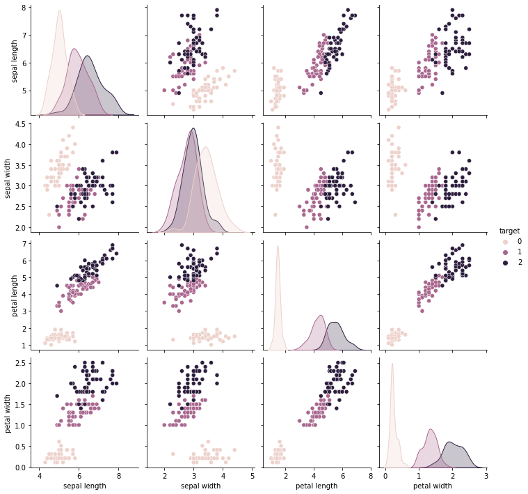

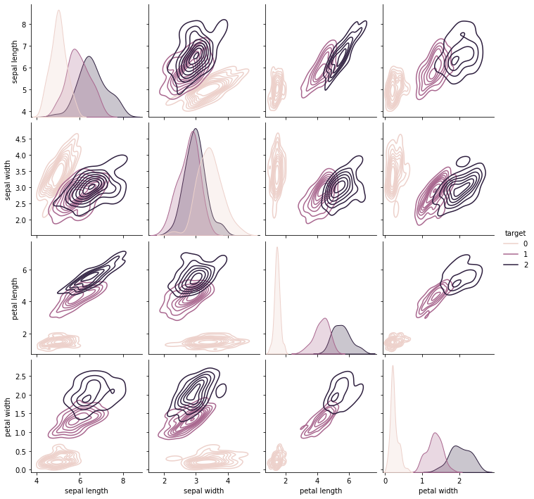
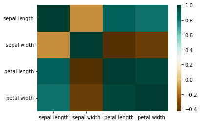
Based on what it is shown, we can see that density based algorithm may work quite while as many of the features look like there are distinct clusters that can uniquely identify the data. While the histogram does show that petal length and petal width can be useful to be used for probability and gaussian based usages. Based on the correlation heatmap, we can see that the petal length and petal width have the highest class correlation as well.

Print Result

The following function is to easily print the result of the models that we are going to demonstrate, in the following sections.

def print_result(model_type:str, model, xtest:iter, ytest:iter, predictions:iter):

    """
    prints results of the models, does not return any values other than printing.

    Parameter
    ---------
    model_type: str
        name of the model, to identify the model

    model: class
        sklearn models

    xtest: iter
        the x test set - test set used to train

    ytest: iter
        the y test set - test set used to test the prediction

    predictions: iter
        the model's output, list of predictions

    """

    # Print and format the name of the model
    print(model_type, end="\n======================================== \n")

    # Print the accuracy
    print("Accuracy: ",end="")
    score = model.score(xtest, ytest)
    print("{:.2%}".format(score),end="\n\n") # format the print, so that only 2 decimal place

    # Print the confusion matrix
    print("Confusion Matrix: ")
    print(confusion_matrix(ytest, predictions), end="\n\n")

    # Print the classification report
    print(classification_report(ytest,predictions),end="\n\n\n")

1.1 Naïve Bayes Classifier [2]

Train a Naïve Bayes classifier in python.

Use your code to fit the data given above.

There are several types of Naïve Bayes classifier in scikit-learn, we can explore the different versions of Naïve Bayes classifier and see which is the better performer.

Gaussian Naive Bayes

Initial/Default Run

# Gaussian Naive Bayes

# Initialize the model
naive_bayes_classifier_gaussian = GaussianNB()

# Fit the data
naive_bayes_classifier_gaussian.fit(X_train, y_train)

# Using the X test, to make predictions
pred_gaussian = naive_bayes_classifier_gaussian.predict(X_test)

# Using y test to compare with the predictions made, print the results
print_result("Gaussian Naive Bayes", naive_bayes_classifier_gaussian, X_test, y_test, pred_gaussian)

Gaussian Naive Bayes
========================================
Accuracy: 95.56%

Confusion Matrix:
[[16  0  0]
 [ 0 16  1]
 [ 0  1 11]]

              precision    recall  f1-score   support

           0       1.00      1.00      1.00        16
           1       0.94      0.94      0.94        17
           2       0.92      0.92      0.92        12

    accuracy                           0.96        45
   macro avg       0.95      0.95      0.95        45
weighted avg       0.96      0.96      0.96        45

Parameters in Gaussian Naive Bayes. Prior Probability

Because GaussianNB() has only got 2 parameters, we can explore can we optimize the model in anyway. The first parameter is the ability to list down the prior probability. By default, it will check for the number of occurrences in the dataset for the given class value or target value. For example, by using the attribute "classprior" on the model above, we can view the prior probability generated by the model.

# Calculating the number of occurrence in each class
dict_count = {}
for count in y_train:
    if count not in dict_count.keys():
        dict_count[count] = 1
    else:
        dict_count[count] += 1

# Print the number of occurrence in each class
print("Class and its occurence:")
print(dict_count, end="\n\n")

# Calculating total occurrence
total = 0
for key in dict_count:
    total += dict_count[key]

print("Total Occurrence:", total)

# Individual Probability
for key in dict_count:
    print("Class " + str(key) + ": " + "{:.4f}".format(dict_count[key]/total))

# Print the prior probability from the model
print()
print("Prior Probability from the Model")
print(naive_bayes_classifier_gaussian.class_prior_)

Class and its occurence:
{1: 33, 0: 34, 2: 38}

Total Occurrence: 105
Class 1: 0.3143
Class 0: 0.3238
Class 2: 0.3619

Prior Probability from the Model
[0.32380952 0.31428571 0.36190476]

Testing Prior Probability

Therefore, if we were to try to keep the prior probability fair, because the dataset has 50 of each of the class value or target value. We will see what the result would be

# Gaussian Naive Bayes with Equal Prior Probability

# Prior Probability
prior_probability = [0.3333, 0.3333, 0.3334] # the total needs to be a 1

# Initialize the model
naive_bayes_classifier_gaussian_prior = GaussianNB(
    priors=prior_probability
)

# Fit the data
naive_bayes_classifier_gaussian_prior.fit(X_train, y_train)

# Using the X test, to make predictions
pred_gaussian_prior = naive_bayes_classifier_gaussian_prior.predict(X_test)

# Using y test to compare with the predictions made, print the results
print_result("Gaussian Naive Bayes with Equal Prior", naive_bayes_classifier_gaussian_prior, X_test, y_test, pred_gaussian_prior)

Gaussian Naive Bayes with Equal Prior
========================================
Accuracy: 95.56%

Confusion Matrix:
[[16  0  0]
 [ 0 16  1]
 [ 0  1 11]]

              precision    recall  f1-score   support

           0       1.00      1.00      1.00        16
           1       0.94      0.94      0.94        17
           2       0.92      0.92      0.92        12

    accuracy                           0.96        45
   macro avg       0.95      0.95      0.95        45
weighted avg       0.96      0.96      0.96        45

Parameters in Gaussian Naive Bayes. Variance Smoothing

Based on the result shown above, there are no difference changing the values of the prior probability. Now let's explore the other parameter, variance smoothing. In the user guide by sklearn, there are two attributes that we can use to observe the changes in the model regarding variance smoothing, Epsilon and the Variance, which is defined as absolute additive value to variances and variance of each feature per class. Given the definition, we should be expecting an increase trend.

# Gaussian Naive Bayes with Variance Smoothing

# List of Variance
# Because the default value is such a small number, we shall test with the values of the following
list_of_variance = [0.01, 0.1, 0.25, 0.5, 1, 3, 5]

for var in list_of_variance:
    # Initialize the model
    naive_bayes_classifier_gaussian_var = GaussianNB(
        var_smoothing = var
    )

    # Fit the data
    naive_bayes_classifier_gaussian_var.fit(X_train, y_train)

    # Using the X test, to make predictions
    pred_gaussian_var = naive_bayes_classifier_gaussian_var.predict(X_test)

    # Print the epsilon and var attribute in the mode
    print("This is the var_: ")
    print(naive_bayes_classifier_gaussian_var.var_, end="\n\n")
    print("This is the epsilon_: ")
    print(naive_bayes_classifier_gaussian_var.epsilon_, end="\n\n")

    # Using y test to compare with the predictions made, print the results
    name = "Gaussian Naive Bayes with Var Smoothing, " + str(var)
    print_result(name, naive_bayes_classifier_gaussian_var, X_test, y_test, pred_gaussian_var)

Code Output

This is the var_:
[[0.15553675 0.18788969 0.05948139 0.04515613]
 [0.34072189 0.11697533 0.28599278 0.06347671]
 [0.4645215  0.12499934 0.33393979 0.10433452]]

This is the epsilon_:
0.03155751473922903

Gaussian Naive Bayes with Var Smoothing - 0.01
========================================
Accuracy: 97.78%

Confusion Matrix:
[[16  0  0]
 [ 0 16  1]
 [ 0  0 12]]

              precision    recall  f1-score   support

           0       1.00      1.00      1.00        16
           1       1.00      0.94      0.97        17
           2       0.92      1.00      0.96        12

    accuracy                           0.98        45
   macro avg       0.97      0.98      0.98        45
weighted avg       0.98      0.98      0.98        45



This is the var_:
[[0.43955439 0.47190733 0.34349902 0.32917376]
 [0.62473952 0.40099296 0.57001041 0.34749434]
 [0.74853914 0.40901698 0.61795742 0.38835216]]

This is the epsilon_:
0.3155751473922903

Gaussian Naive Bayes with Var Smoothing - 0.1
========================================
Accuracy: 97.78%

Confusion Matrix:
[[16  0  0]
 [ 0 17  0]
 [ 0  1 11]]

              precision    recall  f1-score   support

           0       1.00      1.00      1.00        16
           1       0.94      1.00      0.97        17
           2       1.00      0.92      0.96        12

    accuracy                           0.98        45
   macro avg       0.98      0.97      0.98        45
weighted avg       0.98      0.98      0.98        45



This is the var_:
[[0.91291711 0.94527005 0.81686174 0.80253648]
 [1.09810224 0.87435568 1.04337313 0.82085706]
 [1.22190186 0.8823797  1.09132014 0.86171488]]

This is the epsilon_:
0.7889378684807257

Gaussian Naive Bayes with Var Smoothing - 0.25
========================================
Accuracy: 97.78%

Confusion Matrix:
[[16  0  0]
 [ 0 17  0]
 [ 0  1 11]]

              precision    recall  f1-score   support

           0       1.00      1.00      1.00        16
           1       0.94      1.00      0.97        17
           2       1.00      0.92      0.96        12

    accuracy                           0.98        45
   macro avg       0.98      0.97      0.98        45
weighted avg       0.98      0.98      0.98        45



This is the var_:
[[1.70185498 1.73420792 1.60579961 1.59147435]
 [1.88704011 1.66329355 1.832311   1.60979493]
 [2.01083973 1.67131757 1.88025801 1.65065275]]

This is the epsilon_:
1.5778757369614513

Gaussian Naive Bayes with Var Smoothing - 0.5
========================================
Accuracy: 97.78%

Confusion Matrix:
[[16  0  0]
 [ 0 17  0]
 [ 0  1 11]]

              precision    recall  f1-score   support

           0       1.00      1.00      1.00        16
           1       0.94      1.00      0.97        17
           2       1.00      0.92      0.96        12

    accuracy                           0.98        45
   macro avg       0.98      0.97      0.98        45
weighted avg       0.98      0.98      0.98        45



This is the var_:
[[3.27973071 3.31208365 3.18367535 3.16935009]
 [3.46491584 3.24116929 3.41018674 3.18767067]
 [3.58871546 3.2491933  3.45813375 3.22852848]]

This is the epsilon_:
3.1557514739229027

Gaussian Naive Bayes with Var Smoothing - 1
========================================
Accuracy: 95.56%

Confusion Matrix:
[[16  0  0]
 [ 0 15  2]
 [ 0  0 12]]

              precision    recall  f1-score   support

           0       1.00      1.00      1.00        16
           1       1.00      0.88      0.94        17
           2       0.86      1.00      0.92        12

    accuracy                           0.96        45
   macro avg       0.95      0.96      0.95        45
weighted avg       0.96      0.96      0.96        45



This is the var_:
[[9.59123366 9.6235866  9.4951783  9.48085304]
 [9.77641879 9.55267224 9.72168968 9.49917361]
 [9.90021841 9.56069625 9.76963669 9.54003143]]

This is the epsilon_:
9.467254421768708

Gaussian Naive Bayes with Var Smoothing - 3
========================================
Accuracy: 82.22%

Confusion Matrix:
[[16  0  0]
 [ 0  9  8]
 [ 0  0 12]]

              precision    recall  f1-score   support

           0       1.00      1.00      1.00        16
           1       1.00      0.53      0.69        17
           2       0.60      1.00      0.75        12

    accuracy                           0.82        45
   macro avg       0.87      0.84      0.81        45
weighted avg       0.89      0.82      0.82        45



This is the var_:
[[15.90273661 15.93508955 15.80668125 15.79235599]
 [16.08792174 15.86417518 16.03319263 15.81067656]
 [16.21172136 15.8721992  16.08113964 15.85153438]]

This is the epsilon_:
15.778757369614514

Gaussian Naive Bayes with Var Smoothing - 5
========================================
Accuracy: 68.89%

Confusion Matrix:
[[16  0  0]
 [ 0  3 14]
 [ 0  0 12]]

              precision    recall  f1-score   support

           0       1.00      1.00      1.00        16
           1       1.00      0.18      0.30        17
           2       0.46      1.00      0.63        12

    accuracy                           0.69        45
   macro avg       0.82      0.73      0.64        45
weighted avg       0.86      0.69      0.64        45

Results of Variance Smoothing

The result shows that there are improvement that has been achieve by changing away from the default value provided by sklearn, but only by 2.22% difference or 23% improvement, but only by using values of from 0.01 to 0.5. The increase value of variance causes performance to go down, and it can also be seen that the epsilon and variances keep increasing.

This shows that because the variance of each feature has become too large, and has overlap each other. If you noticed, when the variance smoothing value was between 0.01 to 0.5, the variance for each feature, had no overlapping values or at least there are still distinctive among one another. Like when variance smoothing was at 0.01, the first feature has values of 0.43955, 0.62473 and 0.74853. This shows that we can use the first feature to distinguish the different classes. But once the variance smoothing reaches 5, the variance for the first feature was 15.90273, 16.08792, 16.21172. The differences in value become relatively small. Making it difficult for the model to distinguish the different classes.

Multinomial Naive Bayes

Due to some time constraint, we will explore one more Naive Bayes model, as I am overspending time for only one part of the assignment.

In the Multinomial Naive Bayes model, there are 4 parameters, but there are very similar to the one above. There is alpha, force alpha, fit prior and class prior. Based on the documentation, these are what the parameters will do.

alpha. This has a default value of 1, but can be set ourselves. It is a additive smoothing parameter where it tries to avoid the zero probability issue.
force alpha. This has a default value of False, but depending on which version of sklearn we are using. This parameter will force the alpha to a value of 1e-10 if alpha has a smaller value that 1e-10, because when the alpha is too small, it probability will be heavily affected.
fit prior. This has a default value of True. This parameter enables the model to ensure that it uses occurrences to determine the prior probability, if it is false, then we have to provide a value on our own.
class prior. This has a default value of None, we have to provide the value here.

Similar to the above, because setting our own prior probability would not make too much of a difference, we will ignore it this time. But we will be looping a list to see what kind of values will be good for the alpha.

# Multinomial Naive Bayes

# List of alphas
list_of_alphas = [0.001,2, 5, 7, 10, 15, 20]

# Looping the List of Alphas
for al in list_of_alphas:

    # Initialize the Model with the parameters
    naive_bayes_classifier_multinomial = MultinomialNB(
        alpha = al,
        fit_prior = True
    )

    # Fitting the data
    naive_bayes_classifier_multinomial.fit(X_train, y_train)

    # Using the model to predict
    pred_multinomial = naive_bayes_classifier_multinomial.predict(X_test)

    # Set the name for every different parameter
    name = "Multinomial Naive Bayes - alpha: " + str(al)

    # Printing the result
    print_result(name, naive_bayes_classifier_multinomial, X_test, y_test, pred_multinomial)

Code Output

Multinomial Naive Bayes - alpha: 0.001
========================================
Accuracy: 68.89%

Confusion Matrix:
[[16  0  0]
 [ 0  3 14]
 [ 0  0 12]]

              precision    recall  f1-score   support

           0       1.00      1.00      1.00        16
           1       1.00      0.18      0.30        17
           2       0.46      1.00      0.63        12

    accuracy                           0.69        45
   macro avg       0.82      0.73      0.64        45
weighted avg       0.86      0.69      0.64        45



Multinomial Naive Bayes - alpha: 2
========================================
Accuracy: 68.89%

Confusion Matrix:
[[16  0  0]
 [ 0  3 14]
 [ 0  0 12]]

              precision    recall  f1-score   support

           0       1.00      1.00      1.00        16
           1       1.00      0.18      0.30        17
           2       0.46      1.00      0.63        12

    accuracy                           0.69        45
   macro avg       0.82      0.73      0.64        45
weighted avg       0.86      0.69      0.64        45



Multinomial Naive Bayes - alpha: 5
========================================
Accuracy: 68.89%

Confusion Matrix:
[[16  0  0]
 [ 0  3 14]
 [ 0  0 12]]

              precision    recall  f1-score   support

           0       1.00      1.00      1.00        16
           1       1.00      0.18      0.30        17
           2       0.46      1.00      0.63        12

    accuracy                           0.69        45
   macro avg       0.82      0.73      0.64        45
weighted avg       0.86      0.69      0.64        45



Multinomial Naive Bayes - alpha: 7
========================================
Accuracy: 71.11%

Confusion Matrix:
[[16  0  0]
 [ 0  4 13]
 [ 0  0 12]]

              precision    recall  f1-score   support

           0       1.00      1.00      1.00        16
           1       1.00      0.24      0.38        17
           2       0.48      1.00      0.65        12

    accuracy                           0.71        45
   macro avg       0.83      0.75      0.68        45
weighted avg       0.86      0.71      0.67        45



Multinomial Naive Bayes - alpha: 10
========================================
Accuracy: 71.11%

Confusion Matrix:
[[16  0  0]
 [ 0  4 13]
 [ 0  0 12]]

              precision    recall  f1-score   support

           0       1.00      1.00      1.00        16
           1       1.00      0.24      0.38        17
           2       0.48      1.00      0.65        12

    accuracy                           0.71        45
   macro avg       0.83      0.75      0.68        45
weighted avg       0.86      0.71      0.67        45



Multinomial Naive Bayes - alpha: 15
========================================
Accuracy: 68.89%

Confusion Matrix:
[[16  0  0]
 [ 0  3 14]
 [ 0  0 12]]

              precision    recall  f1-score   support

           0       1.00      1.00      1.00        16
           1       1.00      0.18      0.30        17
           2       0.46      1.00      0.63        12

    accuracy                           0.69        45
   macro avg       0.82      0.73      0.64        45
weighted avg       0.86      0.69      0.64        45



Multinomial Naive Bayes - alpha: 20
========================================
Accuracy: 66.67%

Confusion Matrix:
[[16  0  0]
 [ 0  2 15]
 [ 0  0 12]]

              precision    recall  f1-score   support

           0       1.00      1.00      1.00        16
           1       1.00      0.12      0.21        17
           2       0.44      1.00      0.62        12

    accuracy                           0.67        45
   macro avg       0.81      0.71      0.61        45
weighted avg       0.85      0.67      0.60        45

Result

The result were surprising as it did not perform very well. This could be because multinomial naive bayes may need a large dataset or a dataset that involves more counting based variables or values. It is known to be very good at text classification even though it is a fairly simply model.

It can be seen that the model accuracy increased from the alpha value of 7 and 10, but then starts to drop when the value is 20.

Because the performance of Gaussian Naive Bayes is better than Multinomial Naive Bayes, we will be using the results of Gaussian Naive Bayes to compare.

1.2 Random Forst Classifier [3]

Train a random forest classifier in python. Use your code to fit the data given above.

Evaluate feature performance of the model.

Visualise the feature importance.

Because there are many parameters in the Random Forest Classifier. We shall pick only a few to test out and optimize. The following listed are the ones we will look into.

n_estimators. This has a default value of 100. This is the number of trees in the forest. This parameter in theory, the more trees we have, the more accurate the model will be.
criterion. This has a default value of "gini". There are three options for us to choose, "gini", "entropy" and "log_loss". These are methods that decides how the nodes should be split. Will only be using "gini" and "entropy", as due to the current version of sklearn installed is not up to date.
warm_start. This has a default value of False. This parameter decides if the tree should start anew or reuse the solution of the previous call to fit and add more estimators to the ensemble. Using the concept of weak learners.

There are many other parameters that can be used to tweak, but given the restricted time, we will not be going into detail. Furthermore, the dataset has only got 150 samples. Tweaking the max depth, max leaf node, node size, minimum number samples required to split, minimum sample required to become a leaf, etc, seem time consuming and can be dwell into for longer to be fully optimized. Noted that the bootstrap default value is true, which is something good to have running.

# Random Forest Classifier

# Create list of parameters to be looped
number_of_estimators = [10, 25, 50, 100, 150]
list_of_criterions = ["gini", "entropy"]
warm_start_states = [True, False]

# Looping number of estimators parameters
for num in number_of_estimators:

    # Looping list of criterions
    for cri in list_of_criterions:

        # Looping warm start states
        for wss in warm_start_states:

            # Initializing the model with the paramaters
            random_forest_classifier = RandomForestClassifier(
                random_state = mySeed,
                n_estimators= num,
                criterion= cri,
                warm_start= wss
            )

            # Fitting the training data
            random_forest_classifier.fit(X_train, y_train)

            # Predict the data
            pred_RFC = random_forest_classifier.predict(X_test)

            # Set the name for every run with different parameters
            name = "RandomForestClassifier - " + "numEst: " + str(num) + " | criterion: " + cri + " | warm start: " + str(wss)

            # Print result
            print_result(name, random_forest_classifier, X_test, y_test, pred_RFC)

Code Output

RandomForestClassifier - numEst: 10 | criterion: gini | warm start: True
========================================
Accuracy: 95.56%

Confusion Matrix:
[[16  0  0]
 [ 0 16  1]
 [ 0  1 11]]

              precision    recall  f1-score   support

           0       1.00      1.00      1.00        16
           1       0.94      0.94      0.94        17
           2       0.92      0.92      0.92        12

    accuracy                           0.96        45
   macro avg       0.95      0.95      0.95        45
weighted avg       0.96      0.96      0.96        45



RandomForestClassifier - numEst: 10 | criterion: gini | warm start: False
========================================
Accuracy: 95.56%

Confusion Matrix:
[[16  0  0]
 [ 0 16  1]
 [ 0  1 11]]

              precision    recall  f1-score   support

           0       1.00      1.00      1.00        16
           1       0.94      0.94      0.94        17
           2       0.92      0.92      0.92        12

    accuracy                           0.96        45
   macro avg       0.95      0.95      0.95        45
weighted avg       0.96      0.96      0.96        45



RandomForestClassifier - numEst: 10 | criterion: entropy | warm start: True
========================================
Accuracy: 95.56%

Confusion Matrix:
[[16  0  0]
 [ 0 16  1]
 [ 0  1 11]]

              precision    recall  f1-score   support

           0       1.00      1.00      1.00        16
           1       0.94      0.94      0.94        17
           2       0.92      0.92      0.92        12

    accuracy                           0.96        45
   macro avg       0.95      0.95      0.95        45
weighted avg       0.96      0.96      0.96        45



RandomForestClassifier - numEst: 10 | criterion: entropy | warm start: False
========================================
Accuracy: 95.56%

Confusion Matrix:
[[16  0  0]
 [ 0 16  1]
 [ 0  1 11]]

              precision    recall  f1-score   support

           0       1.00      1.00      1.00        16
           1       0.94      0.94      0.94        17
           2       0.92      0.92      0.92        12

    accuracy                           0.96        45
   macro avg       0.95      0.95      0.95        45
weighted avg       0.96      0.96      0.96        45



RandomForestClassifier - numEst: 25 | criterion: gini | warm start: True
========================================
Accuracy: 95.56%

Confusion Matrix:
[[16  0  0]
 [ 0 16  1]
 [ 0  1 11]]

              precision    recall  f1-score   support

           0       1.00      1.00      1.00        16
           1       0.94      0.94      0.94        17
           2       0.92      0.92      0.92        12

    accuracy                           0.96        45
   macro avg       0.95      0.95      0.95        45
weighted avg       0.96      0.96      0.96        45



RandomForestClassifier - numEst: 25 | criterion: gini | warm start: False
========================================
Accuracy: 95.56%

Confusion Matrix:
[[16  0  0]
 [ 0 16  1]
 [ 0  1 11]]

              precision    recall  f1-score   support

           0       1.00      1.00      1.00        16
           1       0.94      0.94      0.94        17
           2       0.92      0.92      0.92        12

    accuracy                           0.96        45
   macro avg       0.95      0.95      0.95        45
weighted avg       0.96      0.96      0.96        45



RandomForestClassifier - numEst: 25 | criterion: entropy | warm start: True
========================================
Accuracy: 95.56%

Confusion Matrix:
[[16  0  0]
 [ 0 16  1]
 [ 0  1 11]]

              precision    recall  f1-score   support

           0       1.00      1.00      1.00        16
           1       0.94      0.94      0.94        17
           2       0.92      0.92      0.92        12

    accuracy                           0.96        45
   macro avg       0.95      0.95      0.95        45
weighted avg       0.96      0.96      0.96        45



RandomForestClassifier - numEst: 25 | criterion: entropy | warm start: False
========================================
Accuracy: 95.56%

Confusion Matrix:
[[16  0  0]
 [ 0 16  1]
 [ 0  1 11]]

              precision    recall  f1-score   support

           0       1.00      1.00      1.00        16
           1       0.94      0.94      0.94        17
           2       0.92      0.92      0.92        12

    accuracy                           0.96        45
   macro avg       0.95      0.95      0.95        45
weighted avg       0.96      0.96      0.96        45



RandomForestClassifier - numEst: 50 | criterion: gini | warm start: True
========================================
Accuracy: 95.56%

Confusion Matrix:
[[16  0  0]
 [ 0 16  1]
 [ 0  1 11]]

              precision    recall  f1-score   support

           0       1.00      1.00      1.00        16
           1       0.94      0.94      0.94        17
           2       0.92      0.92      0.92        12

    accuracy                           0.96        45
   macro avg       0.95      0.95      0.95        45
weighted avg       0.96      0.96      0.96        45



RandomForestClassifier - numEst: 50 | criterion: gini | warm start: False
========================================
Accuracy: 95.56%

Confusion Matrix:
[[16  0  0]
 [ 0 16  1]
 [ 0  1 11]]

              precision    recall  f1-score   support

           0       1.00      1.00      1.00        16
           1       0.94      0.94      0.94        17
           2       0.92      0.92      0.92        12

    accuracy                           0.96        45
   macro avg       0.95      0.95      0.95        45
weighted avg       0.96      0.96      0.96        45



RandomForestClassifier - numEst: 50 | criterion: entropy | warm start: True
========================================
Accuracy: 97.78%

Confusion Matrix:
[[16  0  0]
 [ 0 16  1]
 [ 0  0 12]]

              precision    recall  f1-score   support

           0       1.00      1.00      1.00        16
           1       1.00      0.94      0.97        17
           2       0.92      1.00      0.96        12

    accuracy                           0.98        45
   macro avg       0.97      0.98      0.98        45
weighted avg       0.98      0.98      0.98        45



RandomForestClassifier - numEst: 50 | criterion: entropy | warm start: False
========================================
Accuracy: 97.78%

Confusion Matrix:
[[16  0  0]
 [ 0 16  1]
 [ 0  0 12]]

              precision    recall  f1-score   support

           0       1.00      1.00      1.00        16
           1       1.00      0.94      0.97        17
           2       0.92      1.00      0.96        12

    accuracy                           0.98        45
   macro avg       0.97      0.98      0.98        45
weighted avg       0.98      0.98      0.98        45



RandomForestClassifier - numEst: 100 | criterion: gini | warm start: True
========================================
Accuracy: 95.56%

Confusion Matrix:
[[16  0  0]
 [ 0 16  1]
 [ 0  1 11]]

              precision    recall  f1-score   support

           0       1.00      1.00      1.00        16
           1       0.94      0.94      0.94        17
           2       0.92      0.92      0.92        12

    accuracy                           0.96        45
   macro avg       0.95      0.95      0.95        45
weighted avg       0.96      0.96      0.96        45



RandomForestClassifier - numEst: 100 | criterion: gini | warm start: False
========================================
Accuracy: 95.56%

Confusion Matrix:
[[16  0  0]
 [ 0 16  1]
 [ 0  1 11]]

              precision    recall  f1-score   support

           0       1.00      1.00      1.00        16
           1       0.94      0.94      0.94        17
           2       0.92      0.92      0.92        12

    accuracy                           0.96        45
   macro avg       0.95      0.95      0.95        45
weighted avg       0.96      0.96      0.96        45



RandomForestClassifier - numEst: 100 | criterion: entropy | warm start: True
========================================
Accuracy: 95.56%

Confusion Matrix:
[[16  0  0]
 [ 0 16  1]
 [ 0  1 11]]

              precision    recall  f1-score   support

           0       1.00      1.00      1.00        16
           1       0.94      0.94      0.94        17
           2       0.92      0.92      0.92        12

    accuracy                           0.96        45
   macro avg       0.95      0.95      0.95        45
weighted avg       0.96      0.96      0.96        45



RandomForestClassifier - numEst: 100 | criterion: entropy | warm start: False
========================================
Accuracy: 95.56%

Confusion Matrix:
[[16  0  0]
 [ 0 16  1]
 [ 0  1 11]]

              precision    recall  f1-score   support

           0       1.00      1.00      1.00        16
           1       0.94      0.94      0.94        17
           2       0.92      0.92      0.92        12

    accuracy                           0.96        45
   macro avg       0.95      0.95      0.95        45
weighted avg       0.96      0.96      0.96        45



RandomForestClassifier - numEst: 150 | criterion: gini | warm start: True
========================================
Accuracy: 95.56%

Confusion Matrix:
[[16  0  0]
 [ 0 16  1]
 [ 0  1 11]]

              precision    recall  f1-score   support

           0       1.00      1.00      1.00        16
           1       0.94      0.94      0.94        17
           2       0.92      0.92      0.92        12

    accuracy                           0.96        45
   macro avg       0.95      0.95      0.95        45
weighted avg       0.96      0.96      0.96        45



RandomForestClassifier - numEst: 150 | criterion: gini | warm start: False
========================================
Accuracy: 95.56%

Confusion Matrix:
[[16  0  0]
 [ 0 16  1]
 [ 0  1 11]]

              precision    recall  f1-score   support

           0       1.00      1.00      1.00        16
           1       0.94      0.94      0.94        17
           2       0.92      0.92      0.92        12

    accuracy                           0.96        45
   macro avg       0.95      0.95      0.95        45
weighted avg       0.96      0.96      0.96        45



RandomForestClassifier - numEst: 150 | criterion: entropy | warm start: True
========================================
Accuracy: 95.56%

Confusion Matrix:
[[16  0  0]
 [ 0 16  1]
 [ 0  1 11]]

              precision    recall  f1-score   support

           0       1.00      1.00      1.00        16
           1       0.94      0.94      0.94        17
           2       0.92      0.92      0.92        12

    accuracy                           0.96        45
   macro avg       0.95      0.95      0.95        45
weighted avg       0.96      0.96      0.96        45



RandomForestClassifier - numEst: 150 | criterion: entropy | warm start: False
========================================
Accuracy: 95.56%

Confusion Matrix:
[[16  0  0]
 [ 0 16  1]
 [ 0  1 11]]

              precision    recall  f1-score   support

           0       1.00      1.00      1.00        16
           1       0.94      0.94      0.94        17
           2       0.92      0.92      0.92        12

    accuracy                           0.96        45
   macro avg       0.95      0.95      0.95        45
weighted avg       0.96      0.96      0.96        45

The parameter with number of estimator of 50, criterion of entropy and regardless whether it is warm start or not, the accuracy was at its highest with these set of parameters. It has one additional correct guess with made it better than the rest. We will now use the value between 50 and 100 to see if there are any point where it is has better performance and also explore feature importance.

# Random Forest Classifier

# Create list of parameters to be looped
number_of_estimators = [50, 55, 60, 65, 70, 80]

# Looping number of estimators parameters
for num in number_of_estimators:
    # Initializing the model with the paramaters
    random_forest_classifier = RandomForestClassifier(
        random_state = mySeed,
        n_estimators= num,
        criterion= "entropy",
    )

    # Fitting the training data
    random_forest_classifier.fit(X_train, y_train)

    # Predict the data
    pred_RFC = random_forest_classifier.predict(X_test)

    # Set the name for every run with different parameters
    name = "RandomForestClassifier - " + "numEst: " + str(num)

    # Print result
    print_result(name, random_forest_classifier, X_test, y_test, pred_RFC)

Code Output

RandomForestClassifier - numEst: 50
========================================
Accuracy: 97.78%

Confusion Matrix:
[[16  0  0]
 [ 0 16  1]
 [ 0  0 12]]

              precision    recall  f1-score   support

           0       1.00      1.00      1.00        16
           1       1.00      0.94      0.97        17
           2       0.92      1.00      0.96        12

    accuracy                           0.98        45
   macro avg       0.97      0.98      0.98        45
weighted avg       0.98      0.98      0.98        45



RandomForestClassifier - numEst: 55
========================================
Accuracy: 95.56%

Confusion Matrix:
[[16  0  0]
 [ 0 16  1]
 [ 0  1 11]]

              precision    recall  f1-score   support

           0       1.00      1.00      1.00        16
           1       0.94      0.94      0.94        17
           2       0.92      0.92      0.92        12

    accuracy                           0.96        45
   macro avg       0.95      0.95      0.95        45
weighted avg       0.96      0.96      0.96        45



RandomForestClassifier - numEst: 60
========================================
Accuracy: 95.56%

Confusion Matrix:
[[16  0  0]
 [ 0 16  1]
 [ 0  1 11]]

              precision    recall  f1-score   support

           0       1.00      1.00      1.00        16
           1       0.94      0.94      0.94        17
           2       0.92      0.92      0.92        12

    accuracy                           0.96        45
   macro avg       0.95      0.95      0.95        45
weighted avg       0.96      0.96      0.96        45



RandomForestClassifier - numEst: 65
========================================
Accuracy: 95.56%

Confusion Matrix:
[[16  0  0]
 [ 0 16  1]
 [ 0  1 11]]

              precision    recall  f1-score   support

           0       1.00      1.00      1.00        16
           1       0.94      0.94      0.94        17
           2       0.92      0.92      0.92        12

    accuracy                           0.96        45
   macro avg       0.95      0.95      0.95        45
weighted avg       0.96      0.96      0.96        45



RandomForestClassifier - numEst: 70
========================================
Accuracy: 95.56%

Confusion Matrix:
[[16  0  0]
 [ 0 16  1]
 [ 0  1 11]]

              precision    recall  f1-score   support

           0       1.00      1.00      1.00        16
           1       0.94      0.94      0.94        17
           2       0.92      0.92      0.92        12

    accuracy                           0.96        45
   macro avg       0.95      0.95      0.95        45
weighted avg       0.96      0.96      0.96        45



RandomForestClassifier - numEst: 80
========================================
Accuracy: 95.56%

Confusion Matrix:
[[16  0  0]
 [ 0 16  1]
 [ 0  1 11]]

              precision    recall  f1-score   support

           0       1.00      1.00      1.00        16
           1       0.94      0.94      0.94        17
           2       0.92      0.92      0.92        12

    accuracy                           0.96        45
   macro avg       0.95      0.95      0.95        45
weighted avg       0.96      0.96      0.96        45

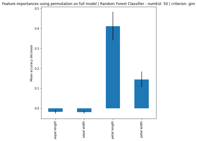
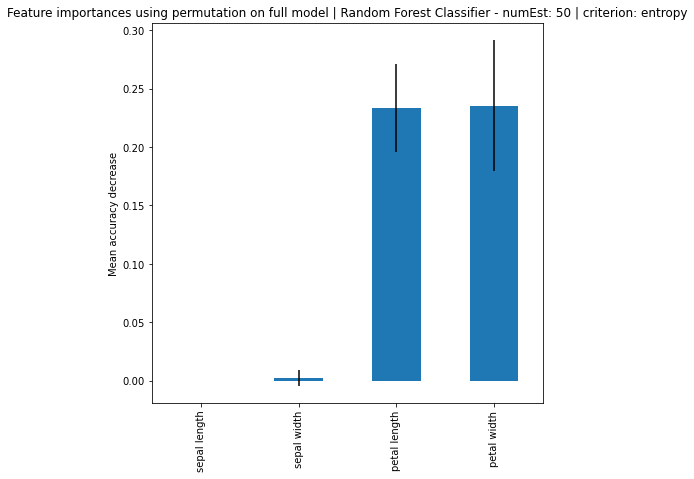
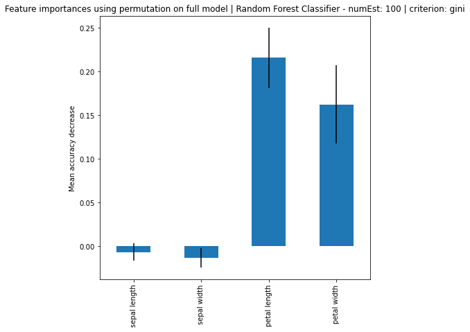
A quick test with number of estimators of 50, 55, 60, 65, 70, 80. At value number 55, the accuracy dropped back to the original. Now we look into the feature importance. In sklearn, there are tutorial and demonstrations regarding feature importance. One way to do it is with Mean Decrease in Impurity (MDI) and another is with feature permutation.

# Random Forest Classifier with Feature importance

# Create list of parameters to be looped
number_of_estimators = [10, 50, 100]
list_of_criterions = ["gini", "entropy"]

# Looping number of estimators parameters
for num in number_of_estimators:
    # Looping the criterions
    for cri in list_of_criterions:
        # Initializing the model with the paramaters
        random_forest_classifier = RandomForestClassifier(
            random_state = mySeed,
            n_estimators= num,
            criterion= cri,
        )

        # Fitting the training data
        random_forest_classifier.fit(X_train, y_train)

        # Predict the data
        pred_RFC = random_forest_classifier.predict(X_test)

        # Set the name for every run with different parameters
        name = "Random Forest Classifier - " + "numEst: " + str(num) + " | criterion: " + cri
        print(name, "===========================")

        # Feature Importance using MDI
        # ---------------------------------
        # Extracting all the feature importance
        importances = random_forest_classifier.feature_importances_
        print("Feature Importance:", importances)

        # Calculate the Standard Deviation for each feature
        rfc_est_importances = [tree.feature_importances_ for tree in random_forest_classifier.estimators_]
        std = np.std(rfc_est_importances, axis=0)
        print("Standard Deviation: ", std)

        # Store importance into series
        forest_importances = pd.Series(importances, index = feature_names)

        # Plot the feature importance and the standard deviation
        fig, ax = plt.subplots(figsize = (7,7))
        forest_importances.plot.bar(yerr=std, ax=ax)
        ax.set_title("Feature importances using MDI | " + name)
        ax.set_ylabel("Mean decrease in impurity")

        # Feature Importance using feature permutation
        # ------------------------------------------------
        # Using the permutation model
        result = permutation_importance(
            random_forest_classifier,
            X_test,
            y_test,
            n_repeats=10,
            random_state=mySeed
        )

        # Store the mean of the all the importances
        rfc_permutated_importances = pd.Series(result.importances_mean, index=feature_names)

        # Plot the feature importances and standard deviation
        fig, ax = plt.subplots(figsize = (7,7))
        rfc_permutated_importances.plot.bar(yerr=result.importances_std, ax=ax)
        ax.set_title("Feature importances using permutation on full model | " + name)
        ax.set_ylabel("Mean accuracy decrease")
        plt.show()

Random Forest Classifier - numEst: 10 | criterion: gini ===========================
Feature Importance: [0.16279096 0.0645915  0.47824496 0.29437258]
Standard Deviation:  [0.17528416 0.09146955 0.22188733 0.15935788]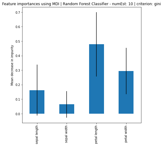

Random Forest Classifier - numEst: 10 | criterion: entropy ===========================
Feature Importance: [0.15221283 0.07886478 0.46957263 0.29934976]
Standard Deviation:  [0.16479341 0.10676639 0.25663494 0.16849768]

Random Forest Classifier - numEst: 50 | criterion: gini ===========================
Feature Importance: [0.06306591 0.03475377 0.48512158 0.41705873]
Standard Deviation:  [0.11483093 0.06516481 0.26416876 0.25654371]

Random Forest Classifier - numEst: 50 | criterion: entropy ===========================
Feature Importance: [0.06524346 0.02754691 0.4601335  0.44707612]
Standard Deviation:  [0.11575326 0.06094211 0.29808099 0.2944902 ]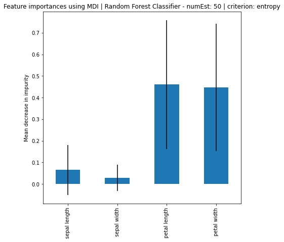

Random Forest Classifier - numEst: 100 | criterion: gini ===========================
Feature Importance: [0.07361742 0.03301872 0.46369241 0.42967146]
Standard Deviation:  [0.13593804 0.06788313 0.29035863 0.28033518]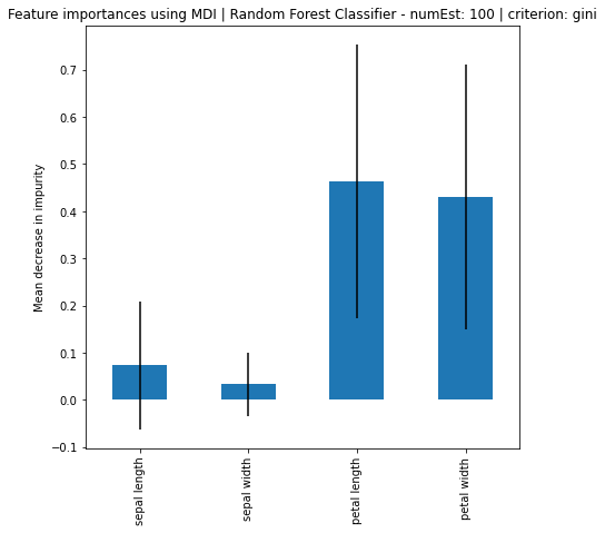

Random Forest Classifier - numEst: 100 | criterion: entropy ===========================
Feature Importance: [0.07751507 0.02765796 0.45062813 0.44419884]
Standard Deviation:  [0.13836613 0.05406896 0.30739594 0.29751664]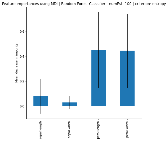

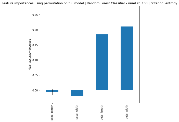
Based on the results, it can be seen that increase in number of estimators, the larger the difference of importance between the features, regardless if using MDI or Feature Permutation. Petal length and petal width is obviously the more important feature where it strongly weight on the final decision. Even using a simple correlation matrix, the petal length and petal width had the highest correlation. Using methods such as feature importance using MDI and feature permutation, only further solidify the point.

1.3 kNN Classifier [2]

Train a kNN classifier in python.

Use your code to fit the data given above.

Similar to Random Forest Classifier where there are quite a number of parameter that can be explored for the model. We will be picking a few of to be testing. The parameters available to pick are as follows.

Number of Neighbours. This has a default value of 5. This will affect how many neighbours will it consider when classifying a data point.
Weights. This has a default value of 'uniform'. We can choose between 'uniform', 'distance' or our own self defined metric. This will affect the decision factor when deciding if the data point belongs to either of the classes. When there is a tie in a the group of neighbours, for example, 5 A and 5 B, then it will use distance between all the data points as a tiebreaker.
Algorithm. This has a default value of 'auto'. We can choose between 'auto', 'ball_tree', 'kd_tree', and 'brute'. 'Auto' will determine if whichever method is the optimal for the given dataset. This is the algorithm that will compute the nearest neighbours.
Metric. This has a default value of 'minkowski' because 'minkowski' can also be manhattan distance and euclidean distance by using diffent p value. Sklearn also allows users to use different predefined distance metrics in their package.
p. This has a default value of 2, which cause the minkowski distance to be euclidean distance. Value of 1 will make it manhattan distance.

We will be testing number of neighbours, weights, and p value, because there are limited choices with the metric and since auto will already be picking an optimal choice based on the dataset, we need not test the other algorithms then.

# Write your code here

# List of Parameters
weights = ['uniform', 'distance']
number_of_neighbours = [x for x in range(3,11)]
p_numbers = [1,2,3,5,10]


# Looping through number of neighbours
for num in number_of_neighbours:
     # Looping through weights
    for w in weights:
        # Looping through p numbers
        for p_num in p_numbers:

            # Initializing the model
            kNN_classifier = KNeighborsClassifier(
                weights = w,
                n_neighbors = num,
                p = p_num
            )

            # Fitting the data
            kNN_classifier.fit(X_train, y_train)

            # Prediction
            pred_knn = kNN_classifier.predict(X_test)

            # Setting the name to display the different parameters every round
            knnName = "kNN Classifier - No of Neigbours: " + str(num) + " | Weights: " + str(w) \
            + " | p: " + str(p_num)

            # Store the score of prediction against the actual value
            score = kNN_classifier.score(X_test, y_test)

            # Print name and score
            print("{} --- {:.3f}% \n".format(knnName, score*100))

            #print_result(knnName, kNN_classifier, X_test, y_test, pred_knn)

Code Output

kNN Classifier - No of Neigbours: 3 | Weights: uniform | p: 1 --- 97.778%

kNN Classifier - No of Neigbours: 3 | Weights: uniform | p: 2 --- 97.778%

kNN Classifier - No of Neigbours: 3 | Weights: uniform | p: 3 --- 97.778%

kNN Classifier - No of Neigbours: 3 | Weights: uniform | p: 5 --- 97.778%

kNN Classifier - No of Neigbours: 3 | Weights: uniform | p: 10 --- 97.778%

kNN Classifier - No of Neigbours: 3 | Weights: distance | p: 1 --- 97.778%

kNN Classifier - No of Neigbours: 3 | Weights: distance | p: 2 --- 97.778%

kNN Classifier - No of Neigbours: 3 | Weights: distance | p: 3 --- 97.778%

kNN Classifier - No of Neigbours: 3 | Weights: distance | p: 5 --- 97.778%

kNN Classifier - No of Neigbours: 3 | Weights: distance | p: 10 --- 97.778%

kNN Classifier - No of Neigbours: 4 | Weights: uniform | p: 1 --- 95.556%

kNN Classifier - No of Neigbours: 4 | Weights: uniform | p: 2 --- 93.333%

kNN Classifier - No of Neigbours: 4 | Weights: uniform | p: 3 --- 95.556%

kNN Classifier - No of Neigbours: 4 | Weights: uniform | p: 5 --- 95.556%

kNN Classifier - No of Neigbours: 4 | Weights: uniform | p: 10 --- 95.556%

kNN Classifier - No of Neigbours: 4 | Weights: distance | p: 1 --- 97.778%

kNN Classifier - No of Neigbours: 4 | Weights: distance | p: 2 --- 97.778%

kNN Classifier - No of Neigbours: 4 | Weights: distance | p: 3 --- 97.778%

kNN Classifier - No of Neigbours: 4 | Weights: distance | p: 5 --- 97.778%

kNN Classifier - No of Neigbours: 4 | Weights: distance | p: 10 --- 97.778%

kNN Classifier - No of Neigbours: 5 | Weights: uniform | p: 1 --- 95.556%

kNN Classifier - No of Neigbours: 5 | Weights: uniform | p: 2 --- 97.778%

kNN Classifier - No of Neigbours: 5 | Weights: uniform | p: 3 --- 100.000%

kNN Classifier - No of Neigbours: 5 | Weights: uniform | p: 5 --- 100.000%

kNN Classifier - No of Neigbours: 5 | Weights: uniform | p: 10 --- 100.000%

kNN Classifier - No of Neigbours: 5 | Weights: distance | p: 1 --- 95.556%

kNN Classifier - No of Neigbours: 5 | Weights: distance | p: 2 --- 97.778%

kNN Classifier - No of Neigbours: 5 | Weights: distance | p: 3 --- 97.778%

kNN Classifier - No of Neigbours: 5 | Weights: distance | p: 5 --- 97.778%

kNN Classifier - No of Neigbours: 5 | Weights: distance | p: 10 --- 100.000%

kNN Classifier - No of Neigbours: 6 | Weights: uniform | p: 1 --- 95.556%

kNN Classifier - No of Neigbours: 6 | Weights: uniform | p: 2 --- 100.000%

kNN Classifier - No of Neigbours: 6 | Weights: uniform | p: 3 --- 97.778%

kNN Classifier - No of Neigbours: 6 | Weights: uniform | p: 5 --- 97.778%

kNN Classifier - No of Neigbours: 6 | Weights: uniform | p: 10 --- 97.778%

kNN Classifier - No of Neigbours: 6 | Weights: distance | p: 1 --- 97.778%

kNN Classifier - No of Neigbours: 6 | Weights: distance | p: 2 --- 97.778%

kNN Classifier - No of Neigbours: 6 | Weights: distance | p: 3 --- 97.778%

kNN Classifier - No of Neigbours: 6 | Weights: distance | p: 5 --- 97.778%

kNN Classifier - No of Neigbours: 6 | Weights: distance | p: 10 --- 97.778%

kNN Classifier - No of Neigbours: 7 | Weights: uniform | p: 1 --- 95.556%

kNN Classifier - No of Neigbours: 7 | Weights: uniform | p: 2 --- 100.000%

kNN Classifier - No of Neigbours: 7 | Weights: uniform | p: 3 --- 100.000%

kNN Classifier - No of Neigbours: 7 | Weights: uniform | p: 5 --- 100.000%

kNN Classifier - No of Neigbours: 7 | Weights: uniform | p: 10 --- 100.000%

kNN Classifier - No of Neigbours: 7 | Weights: distance | p: 1 --- 97.778%

kNN Classifier - No of Neigbours: 7 | Weights: distance | p: 2 --- 97.778%

kNN Classifier - No of Neigbours: 7 | Weights: distance | p: 3 --- 97.778%

kNN Classifier - No of Neigbours: 7 | Weights: distance | p: 5 --- 97.778%

kNN Classifier - No of Neigbours: 7 | Weights: distance | p: 10 --- 100.000%

kNN Classifier - No of Neigbours: 8 | Weights: uniform | p: 1 --- 95.556%

kNN Classifier - No of Neigbours: 8 | Weights: uniform | p: 2 --- 100.000%

kNN Classifier - No of Neigbours: 8 | Weights: uniform | p: 3 --- 100.000%

kNN Classifier - No of Neigbours: 8 | Weights: uniform | p: 5 --- 100.000%

kNN Classifier - No of Neigbours: 8 | Weights: uniform | p: 10 --- 100.000%

kNN Classifier - No of Neigbours: 8 | Weights: distance | p: 1 --- 97.778%

kNN Classifier - No of Neigbours: 8 | Weights: distance | p: 2 --- 97.778%

kNN Classifier - No of Neigbours: 8 | Weights: distance | p: 3 --- 97.778%

kNN Classifier - No of Neigbours: 8 | Weights: distance | p: 5 --- 97.778%

kNN Classifier - No of Neigbours: 8 | Weights: distance | p: 10 --- 97.778%

kNN Classifier - No of Neigbours: 9 | Weights: uniform | p: 1 --- 97.778%

kNN Classifier - No of Neigbours: 9 | Weights: uniform | p: 2 --- 97.778%

kNN Classifier - No of Neigbours: 9 | Weights: uniform | p: 3 --- 97.778%

kNN Classifier - No of Neigbours: 9 | Weights: uniform | p: 5 --- 97.778%

kNN Classifier - No of Neigbours: 9 | Weights: uniform | p: 10 --- 97.778%

kNN Classifier - No of Neigbours: 9 | Weights: distance | p: 1 --- 97.778%

kNN Classifier - No of Neigbours: 9 | Weights: distance | p: 2 --- 97.778%

kNN Classifier - No of Neigbours: 9 | Weights: distance | p: 3 --- 97.778%

kNN Classifier - No of Neigbours: 9 | Weights: distance | p: 5 --- 97.778%

kNN Classifier - No of Neigbours: 9 | Weights: distance | p: 10 --- 97.778%

kNN Classifier - No of Neigbours: 10 | Weights: uniform | p: 1 --- 100.000%

kNN Classifier - No of Neigbours: 10 | Weights: uniform | p: 2 --- 97.778%

kNN Classifier - No of Neigbours: 10 | Weights: uniform | p: 3 --- 97.778%

kNN Classifier - No of Neigbours: 10 | Weights: uniform | p: 5 --- 95.556%

kNN Classifier - No of Neigbours: 10 | Weights: uniform | p: 10 --- 95.556%

kNN Classifier - No of Neigbours: 10 | Weights: distance | p: 1 --- 97.778%

kNN Classifier - No of Neigbours: 10 | Weights: distance | p: 2 --- 97.778%

kNN Classifier - No of Neigbours: 10 | Weights: distance | p: 3 --- 97.778%

kNN Classifier - No of Neigbours: 10 | Weights: distance | p: 5 --- 97.778%

kNN Classifier - No of Neigbours: 10 | Weights: distance | p: 10 --- 97.778%

Result

Based on the result, regardless of the parameters used, 97.78% accuracy is the highest occurrence, with some occasional 100% and 1 instance of a 93.33%.

2 Code Report [6 marks total]

In a markdown box, write a short report (no more than 500 words) that describes the workings of your code.

Code Report

I think that I have been describing the workings of my code throughout and describing the outputs as well, with all the markdown cells in place. Additionally, I have place comments in the code to describe what was done in the code. Explaining it fully here will only be repetitive and redundant but a summary will be given.

I have split the data into training and test set by using sklearn train test split function, training set of 70% and testing set of 30%. I have also used seaborn library to visualize the data initially to have an idea how the data was plotted and distributed. Then also visualize the correlation using heatmap and it can be seen that 'petal width' and 'petal length' features were highly correlated. Furthermore, in the iris dataset description, it is also mentioned that 'petal width' and 'petal length' have high class correlation.

Then, in Naive Bayes Classifier, tested out Gaussian and Multinomial Naive Bayes. Gaussian was clearly the better choice as it was definitely not the right dataset for Multinomial Naive Bayes. This is because, as shown in the data visualization, that features are had clear distinctive histograms, especially for 'petal width' and 'petal length' and it was gaussian in nature. Multinomial will be better on discrete and distinctive data that has to do with frequency.

Next, exploring the parameters in Random Forest to pick the set that can have the highest performance. Found a specific set of parameter that perform best by 1 extra correct prediction, and then the rest of the parameters are the same. Then, based on what is shown in sklearn, performed feature importance using mean decrease in impurity and feature permutation.

Lastly, for the kNN classifier, parameters were explore similarly to the Random Forest Classifier, to find out which set of parameters performs best. As for kNN, regardless of the parameters chosen, it was performing very well. There were many instances of 97.78% accuracy and occasional 100%.

3 Model Questions [14 marks total]

Please answer the following questions relating to your classifiers.

3.1 Naïves Bayes Questions [4]

Why do zero probabilities in our Naïve Bayes model cause problems?

How can we avoid the problem of zero probabilities in our Naïve Bayes model?

Please answer in the cell below.

Why do zero probabilities in our Naïve Bayes model cause problems?

Because the Naïve Bayes models rely on probability concepts. If any of the variables, instances, features have a probability of 0, it will nullify that particular prediction or cancel it entirely. This causes misclassifications.

For example, assuming we are using Multinomial Naive Bayes, where given that events $\large A$ and $\large B$ have prior probabilities of 0.6 and 0.4 respectively, consisting of values of $\large a$ , $\large b$ and $\large c$ with different sets of probabilities.

Event $\large A$ $\{a = 0.40, b = 0.50, c = 0.10 \}$ , with a frequency of $\{a = 4, b = 5, c = 1\}$

Event $\large B$ $\{a = 0.00, b = 0.20, c = 0.80 \}$ with a frequency of $\{a = 0, b = 2, c = 8\}$

Given that we have a sample of $\large \{ b,b,b,c\}$ , which will be called sample $\text{x}$ .

$P(A|\text{x}) = \text{Prior Probability * P(A|b) * P(A|b) * P(A|b) * P(A|c)} = 0.60 * 0.40 * 0.40 * 0.40 * 0.10 = 0.0038$

$P(B|\text{x}) = \text{Prior Probability * P(B|b) * P(B|b) * P(B|b) * P(B|c)} = 0.40 * 0.20 * 0.20 * 0.20 * 0.80 = 0.0026$

Because the value of $P(A|\text{x})$ is higher than $P(B|\text{x})$ , we can conclude that there is a high probability that sample $\text{x}$ is belong to or classified as Event $\large A$

Given that we have a sample of $\large \{ c,c,c,a\}$ , which will be called sample $\text{y}$ . We can assume that it should belong to or classified under Event $\large B$ , but because of a zero probability for $P(B|a)$ , it will wrongly classify it as Event $\large A$ , as shown below.

$P(A|\text{x}) = \text{Prior Probability _ P(A|c) _ P(A|c) _ P(A|c) _ P(A|a)} = 0.60 _ 0.10 _ 0.10 _ 0.10 _ 0.40 = 0.00024 $

$P(B|\text{x}) = \text{Prior Probability _ P(B|c) _ P(B|c) _ P(B|c) _ P(B|a)} = 0.40 _ 0.80 _ 0.80 _ 0.80 _ 0.00 = 0.00000 $

Because the value of $P(A|x)$ is higher than $P(B|x)$ , we can conclude that there is a high probability that sample $\text{x}$ is belong to or classified as Event $\large A$ . This is the biggest reason why, zero probability will affect the performance of the model, as it cancels out the entire formula. This is not only a problem in this model/algorithm but several machine learning algorithm like neural network and its importance of weights. A value of zero can completely disable a neuron in a layer.

How can we avoid the problem of zero probabilities in our Naïve Bayes model?

The solution to this is to have a bias amount or pseudocounts or also known as additive smoothing, which is usually represented by the symbol $\large \alpha$ . This value will be placed into all the variables or features. The value $\large \alpha$ can be set to any value but usually it is either 1 or less than 1. Sometimes, calculations like mean, variance or standard deviation could be used for the $\large \alpha$ as well, depending on the use case and dataset. For example, using the example above where the classification was wrong. Because now that we have add one into the frequency, the probability of the samples will have to change, but it is still closely similar.

Event $\large A$ $\{a = 0.385, b = 0.462, c = 0.153 \}$ , with a frequency of $\{a = 5, b = 6, c = 2\}$

Event $\large B$ $\{a = 0.077, b = 0.231, c = 0.692 \}$ with a frequency of $\{a = 1, b = 3, c = 9\}$

Now with the new updated values, we can now properly calculate the sample $\large \text{x}$ of $\large \{ c,c,c,a \}$ .

$P(A|\text{x}) = \text{Prior Probability _ P(A|c) _ P(A|c) _ P(A|c) _ P(A|a)} = 0.60 _ 0.153 _ 0.153 _ 0.153 _ 0.385 = 0.00082 $

$P(B|\text{x}) = \text{Prior Probability _ P(B|c) _ P(B|c) _ P(B|c) _ P(B|a)} = 0.40 _ 0.692 _ 0.692 _ 0.692 _ 0.077 = 0.01021 $

With the $\large \alpha$ , or the pseudocount, added to the frequency of the sample, to ensure that there is no zero, we can conclude that there is a high probability that sample $\text{y}$ is belong to or classified as Event $\large B$

3.2 Random Forest Questions [6]

Which feature is the most important from your random forest classifier?

Can any features be removed to increase accuracy of the model, if so which features?

Explain why it would be useful to remove these features.

Please answer in the cell below.

# Using only the top two features for Random Forest Classifier

# Dropping the 2 features that have lower feature importance
df_x_2_features = df_x.drop(columns = ['sepal length', 'sepal width'])

# Training and Test Data split based on the dropped data
X_train_2, X_test_2, y_train_2, y_test_2 = train_test_split(
    df_x_2_features, y, test_size=0.3, random_state=mySeed)

# List of variables to loop
number_of_estimators_2 = [1,2,3,50]

# Looping throught the variable
for num2 in number_of_estimators_2:
    # Initialize the Model
    random_forest_classifier_2 = RandomForestClassifier(
            random_state = mySeed,
            n_estimators= num2,
            criterion= "entropy",
        )

    # Fitting the training data
    random_forest_classifier_2.fit(X_train_2, y_train_2)

    # Predict the data
    pred_RFC = random_forest_classifier_2.predict(X_test_2)

    # Set the name for every run with different parameters
    name = "RandomForestClassifier - " + "numEst: " + str(num2)

    # Print result
    print_result(name, random_forest_classifier_2, X_test_2, y_test_2, pred_RFC)

Code Output

RandomForestClassifier - numEst: 1
========================================
Accuracy: 95.56%

Confusion Matrix:
[[16  0  0]
 [ 0 16  1]
 [ 0  1 11]]

              precision    recall  f1-score   support

           0       1.00      1.00      1.00        16
           1       0.94      0.94      0.94        17
           2       0.92      0.92      0.92        12

    accuracy                           0.96        45
   macro avg       0.95      0.95      0.95        45
weighted avg       0.96      0.96      0.96        45



RandomForestClassifier - numEst: 2
========================================
Accuracy: 95.56%

Confusion Matrix:
[[16  0  0]
 [ 0 16  1]
 [ 0  1 11]]

              precision    recall  f1-score   support

           0       1.00      1.00      1.00        16
           1       0.94      0.94      0.94        17
           2       0.92      0.92      0.92        12

    accuracy                           0.96        45
   macro avg       0.95      0.95      0.95        45
weighted avg       0.96      0.96      0.96        45



RandomForestClassifier - numEst: 3
========================================
Accuracy: 97.78%

Confusion Matrix:
[[16  0  0]
 [ 0 16  1]
 [ 0  0 12]]

              precision    recall  f1-score   support

           0       1.00      1.00      1.00        16
           1       1.00      0.94      0.97        17
           2       0.92      1.00      0.96        12

    accuracy                           0.98        45
   macro avg       0.97      0.98      0.98        45
weighted avg       0.98      0.98      0.98        45



RandomForestClassifier - numEst: 50
========================================
Accuracy: 97.78%

Confusion Matrix:
[[16  0  0]
 [ 0 16  1]
 [ 0  0 12]]

              precision    recall  f1-score   support

           0       1.00      1.00      1.00        16
           1       1.00      0.94      0.97        17
           2       0.92      1.00      0.96        12

    accuracy                           0.98        45
   macro avg       0.97      0.98      0.98        45
weighted avg       0.98      0.98      0.98        45

Which feature is the most important from your random forest classifier?

Petal width and petal length is the most important, based on the feature importance process, which have consistently shown that it is always significantly higher than the other two, as well as based on the correlation heatmap.

Can any features be removed to increase accuracy of the model, if so which features?

Yes, based on the code shown above, once we dropped the other two remaining column 'sepal length' and 'sepal width', the performance still did very well. In fact, it was performing every bit the same as the one shown in the Random Forest Classifier section. We have chosen to use no of estimator of 1, 2, 3, 50. This is because only now I have realized that because this dataset has so little features, the no of estimators should not be too high. Even so, based on the result when using only 1 and 2 estimators, the accuracy is still 95.56% and 3 and 50 estimators, it was at 97.78%

Explain why it would be useful to remove these features

Removing features are useful if there are resource constraints put in place. For example, needing the model to be quick. If there is a requirement that we need to keep updating the model every hour and as quick as possible when new data is to be fed into the model. Having lesser features would definitely be beneficial as it has lesser calculations to consider. Another example would be hardware limitations stopping the model to use many features. In such cases, finding out the features that can classify, identify or function effectively, can allow the model to run on lower level hardware. If using all features achieving 90% accuracy but using 3 features can already land you 85%, assuming 85% accuracy is enough, then clearly, picking the one with less features during hardware limitations would make sense. Currently, we are only using a dataset with 4 features and 150 rows of data. If the dataset is any bigger, feature reduction and selection may come more important. Even as shown above, by reducing the feature to 2 features, the accuracy still remain as high as using 4 features.

3.3 kNN Questions [4]

Do you think the kNN classifier is best suited to the iris dataset?

What ideal qualities would the most appropriate dataset display?

Please answer in the cell below.

Do you think the kNN classifier is best suited to the iris dataset?

Based on the best results shown by the model, I think that the kNN Classifier model is very suited for the iris dataset. Another guess that it is suitable is as shown in the visualizing the data, we can see that the features are very distinctly apart from each other, especially the petal length and petal width. Because of this, grouping data points based on the features are a lot easier for the model.

What ideal qualities would the most appropriate dataset display?

As shown in the illustration for petal length and petal width where data is distinctly apart. Features that can alone or in combination of other feature that can unique identify the target value.

4 Comparing Models [18 marks total]

Please answer the following questions comparing your classifiers.

4.1 Compare each model [3]

What differences do you see between your Naïve Bayes classifier, your random forest classifier, and your kNN classifier?

# Test the duration for the models

import time # need this to get current time

# Random Forest Classifier
# -----------------------------------

# Initialize the model - Based on best performing parameters above
rfc = RandomForestClassifier(
    n_estimators= 3,
    criterion="entropy"
)

# Store current time for start time
start_time = time.time()

# Fit the data
rfc.fit(X_train, y_train)

# Print and predict the result
print_result("RandomForestClassifier", rfc, X_test, y_test,rfc.predict(X_test))

# Store current time for end time, difference of end time and start time for duration
duration = time.time() - start_time

# Print duration
print("Random Forest Classifier Duration: ", duration, end="\n\n\n")


# kNN Classifier
# --------------------------

# Initialize the model - Based on best performing parameters above
kNN = KNeighborsClassifier(
    n_neighbors= 5,
    weights='uniform',
    p = 3
)

# Store current time for start time
start_time = time.time()

# Fit the data
kNN.fit(X_train, y_train)

# Print and predict the result
print_result("KNeighborsClassifier", kNN, X_test, y_test, kNN.predict(X_test))

# Store current time for end time, difference of end time and start time for duration
duration = time.time() - start_time

# Print duration
print("KNeighborsClassifier Duration: ", duration)


# Gaussian NB
# ------------------------

# Initialize the model - Based on best performing parameters above
gnb = GaussianNB(
    var_smoothing = 0.1
)

# Store current time for start time
start_time = time.time()

# Fit the data
gnb.fit(X_train, y_train)

# Print and predict the result
print_result("GaussianNB", gnb, X_test, y_test, gnb.predict(X_test))

# Store current time for end time, difference of end time and start time for duration
duration = time.time() - start_time

# Print duration
print("GaussianNB Duration: ", duration)

Code Output

RandomForestClassifier
========================================
Accuracy: 97.78%

Confusion Matrix:
[[16  0  0]
 [ 0 16  1]
 [ 0  0 12]]

              precision    recall  f1-score   support

           0       1.00      1.00      1.00        16
           1       1.00      0.94      0.97        17
           2       0.92      1.00      0.96        12

    accuracy                           0.98        45
   macro avg       0.97      0.98      0.98        45
weighted avg       0.98      0.98      0.98        45



Random Forest Classifier Duration:  0.008522987365722656


KNeighborsClassifier
========================================
Accuracy: 100.00%

Confusion Matrix:
[[16  0  0]
 [ 0 17  0]
 [ 0  0 12]]

              precision    recall  f1-score   support

           0       1.00      1.00      1.00        16
           1       1.00      1.00      1.00        17
           2       1.00      1.00      1.00        12

    accuracy                           1.00        45
   macro avg       1.00      1.00      1.00        45
weighted avg       1.00      1.00      1.00        45



KNeighborsClassifier Duration:  0.005998849868774414
GaussianNB
========================================
Accuracy: 97.78%

Confusion Matrix:
[[16  0  0]
 [ 0 17  0]
 [ 0  1 11]]

              precision    recall  f1-score   support

           0       1.00      1.00      1.00        16
           1       0.94      1.00      0.97        17
           2       1.00      0.92      0.96        12

    accuracy                           0.98        45
   macro avg       0.98      0.97      0.98        45
weighted avg       0.98      0.98      0.98        45



GaussianNB Duration:  0.0040738582611083984

What differences do you see between your Naïve Bayes classifier, your random forest classifier, and your kNN classifier?

Naive Bayes Classifier uses the concept of probability very heavily, random forest classifier uses concepts on bootstrapping, using many trials and feature importance, and kNN classifier is distance based and ideal for grouping. The amount of parameters there are for Naive Bayes is comparatively lesser than the ones for Random Forest and kNN classifier. Random Forest Classifier took the longest out of all the models. I have recreated the best performing models and use time library to get current time, and try to accurately gauge and measure the duration for each of the model, just so to confirm it with quantitative measure.

4.2 Accuracy [6]

Can you explain why there are differences in accuracy between the three classifiers?

Currently, the iris dataset used for the assignment, the accuracy differences are not big enough to consider them differences. They could also be overfitted and hence all the accuracy is are almost at maximum. The biggest difference out of all the model is Multinomial Naive Bayes compared to the other 3 models. This is also because the Multinomial Naive Bayes model is known to be better on text classification situations and datasets. Therefore, it is more like the wrong usage of a model that cause it to have difference in the accuracy compared to all the model. The highest achieved was 70% from what I have done. The kNN model performed best as mentioned above, is that because the features of the dataset seem easily distinguishable. Even for Gaussian Naive Bayes, it was performing very good because the features exhibit gaussian distribution properties, even though two of them had overlaps, but the other two features were very distinctive.

4.3 Appropriate Use [9]

When would it be appropriate to use each different classifier?

Reference real-world situations and examples of specific data sets and explain why that classifier would be most appropriate for that use-case.

We will use some of the real world dataset that is provided by sklearn to compare and see the suitability of the models.

Gaussian Naive Bayes Model is useful if the dataset is known to be normally distributed or distributed similarly to it. Gaussian Naive Bayes should be the fastest among the 3 models here but it may require more preprocessing to try to change the features into gaussian-like properties.

Multinomial Naive Bayes Model is useful for text based problems and frequency related data. In real world use, it is useful for Natural Language Processig.

Random Forest Classifier is useful in many cases due to its ability to bootstrap and weight features accordingly. Its performance is dependant on the hyper parameter that is set, but it is still one of the most flexible model due to it being able to accept many types of data as well. It does not need the feature to only be numeric or probabilistic or continuous etc.

kNN is a simple and effective algorithm that can be used easily and it is considered non-parametric in nature due to other than the value of k, there are not many hyper parameters required to tune, but kNN does not scale as well as the rest when the dataset gets larger, which means it does not work well with large datasets. It may still be able to be used on a large dataset and still perform, but it will require time.

We will be using some of the models for the dataset that has been chosen, shown below, and explanation will be done.

# Import the Forest Covertypes Datasets

from sklearn.datasets import fetch_covtype

# Print the info of the dataset
print(fetch_covtype().DESCR)

# Storing the data and target values for fetch_covtype
X_cov = fetch_covtype().data
y_cov = fetch_covtype().target

# Train Test Split the Cov Dataset
X_cov_train, X_cov_test, y_cov_train, y_cov_test = train_test_split(X_cov, y_cov, test_size=0.2, random_state=mySeed)

.. _covtype_dataset:

Forest covertypes
-----------------

The samples in this dataset correspond to 30×30m patches of forest in the US,
collected for the task of predicting each patch's cover type,
i.e. the dominant species of tree.
There are seven covertypes, making this a multiclass classification problem.
Each sample has 54 features, described on the
`dataset's homepage `__.
Some of the features are boolean indicators,
while others are discrete or continuous measurements.

**Data Set Characteristics:**

    =================   ============
    Classes                        7
    Samples total             581012
    Dimensionality                54
    Features                     int
    =================   ============

:func:`sklearn.datasets.fetch_covtype` will load the covertype dataset;
it returns a dictionary-like 'Bunch' object
with the feature matrix in the ``data`` member
and the target values in ``target``. If optional argument 'as_frame' is
set to 'True', it will return ``data`` and ``target`` as pandas
data frame, and there will be an additional member ``frame`` as well.
The dataset will be downloaded from the web if necessary.

Note that no pre-processing is done. To improve the accuracy of the test belows, I know I should be alter, filter and appropriately modify the data for the model.

The forest covertypes dataset can be used as a good showcase that Random Forest Classifier can handle dataset with higher number of features as compared to kNN.

# Using the fetch_covtype dataset with Random Forest Classifier

# List of estimators to test and loop
list_of_estimators = [18, 27, 54, 114, 216] # Because there are 54 features in the dataset, the estimators chosen are multiples of 54

# Looping through the list of estimators
for est in list_of_estimators:

    # Initialize the class and parameter
    rfc = RandomForestClassifier(
        n_estimators = est
    )

    # Store current time for start time
    start_time = time.time()

    # Fit the data
    rfc.fit(X_cov_train, y_cov_train)

    # Set the name for every loop
    name = "Random Forest Classifier with Cov Dataset: numEst -  " + str(est)

    # Print and predict the results
    print_result(name, rfc, X_cov_test, y_cov_test, rfc.predict(X_cov_test))

    # Store current time for end time, difference of end time and start time for duration
    duration = time.time() - start_time
    print("{} Duration: {:.2f} seconds".format(name, duration))

Code Output

Random Forest Classifier with Cov Dataset: numEst -  18
========================================
Accuracy: 94.98%

Confusion Matrix:
[[39997  2130     0     0     9     8    77]
 [ 1774 54779   106     2    71    66    22]
 [    2   125  6768    24     9   134     0]
 [    0     0    69   469     0    17     0]
 [   36   394    21     0  1452    11     0]
 [    4   115   316    20     4  3047     0]
 [  234    30     0     0     0     0  3861]]

              precision    recall  f1-score   support

           1       0.95      0.95      0.95     42221
           2       0.95      0.96      0.96     56820
           3       0.93      0.96      0.94      7062
           4       0.91      0.85      0.88       555
           5       0.94      0.76      0.84      1914
           6       0.93      0.87      0.90      3506
           7       0.97      0.94      0.96      4125

    accuracy                           0.95    116203
   macro avg       0.94      0.90      0.92    116203
weighted avg       0.95      0.95      0.95    116203



Random Forest Classifier with Cov Dataset: numEst -  18 Duration: 15.13 seconds
Random Forest Classifier with Cov Dataset: numEst -  27
========================================
Accuracy: 95.27%

Confusion Matrix:
[[39825  2288     1     0    11     6    90]
 [ 1413 55143   103     2    59    76    24]
 [    0   100  6789    30     6   137     0]
 [    0     0    68   472     0    15     0]
 [   35   371    31     0  1466    11     0]
 [    5    98   251    15     4  3133     0]
 [  213    29     0     0     0     0  3883]]

              precision    recall  f1-score   support

           1       0.96      0.94      0.95     42221
           2       0.95      0.97      0.96     56820
           3       0.94      0.96      0.95      7062
           4       0.91      0.85      0.88       555
           5       0.95      0.77      0.85      1914
           6       0.93      0.89      0.91      3506
           7       0.97      0.94      0.96      4125

    accuracy                           0.95    116203
   macro avg       0.94      0.90      0.92    116203
weighted avg       0.95      0.95      0.95    116203



Random Forest Classifier with Cov Dataset: numEst -  27 Duration: 21.15 seconds
Random Forest Classifier with Cov Dataset: numEst -  54
========================================
Accuracy: 95.51%

Confusion Matrix:
[[39978  2142     0     0    10     5    86]
 [ 1387 55192    97     0    62    60    22]
 [    2   103  6805    27     6   119     0]
 [    0     0    58   481     0    16     0]
 [   27   365    23     0  1491     8     0]
 [    6    98   237    18     5  3142     0]
 [  210    22     0     0     0     0  3893]]

              precision    recall  f1-score   support

           1       0.96      0.95      0.95     42221
           2       0.95      0.97      0.96     56820
           3       0.94      0.96      0.95      7062
           4       0.91      0.87      0.89       555
           5       0.95      0.78      0.85      1914
           6       0.94      0.90      0.92      3506
           7       0.97      0.94      0.96      4125

    accuracy                           0.96    116203
   macro avg       0.95      0.91      0.93    116203
weighted avg       0.96      0.96      0.95    116203



Random Forest Classifier with Cov Dataset: numEst -  54 Duration: 41.56 seconds
Random Forest Classifier with Cov Dataset: numEst -  114
========================================
Accuracy: 95.61%

Confusion Matrix:
[[39975  2152     1     0     9     5    79]
 [ 1273 55305   101     1    58    60    22]
 [    0    94  6807    26     7   128     0]
 [    0     0    64   477     0    14     0]
 [   25   371    20     0  1486    12     0]
 [    5    98   234    16     3  3150     0]
 [  193    26     0     0     0     0  3906]]

              precision    recall  f1-score   support

           1       0.96      0.95      0.96     42221
           2       0.95      0.97      0.96     56820
           3       0.94      0.96      0.95      7062
           4       0.92      0.86      0.89       555
           5       0.95      0.78      0.85      1914
           6       0.93      0.90      0.92      3506
           7       0.97      0.95      0.96      4125

    accuracy                           0.96    116203
   macro avg       0.95      0.91      0.93    116203
weighted avg       0.96      0.96      0.96    116203



Random Forest Classifier with Cov Dataset: numEst -  114 Duration: 91.15 seconds
Random Forest Classifier with Cov Dataset: numEst -  216
========================================
Accuracy: 95.62%

Confusion Matrix:
[[39923  2199     0     0    11     3    85]
 [ 1239 55338    98     0    62    61    22]
 [    0    96  6806    26     7   127     0]
 [    0     0    57   482     0    16     0]
 [   27   350    21     0  1503    13     0]
 [    5    90   233    18     4  3156     0]
 [  197    25     0     0     0     0  3903]]

              precision    recall  f1-score   support

           1       0.96      0.95      0.95     42221
           2       0.95      0.97      0.96     56820
           3       0.94      0.96      0.95      7062
           4       0.92      0.87      0.89       555
           5       0.95      0.79      0.86      1914
           6       0.93      0.90      0.92      3506
           7       0.97      0.95      0.96      4125

    accuracy                           0.96    116203
   macro avg       0.95      0.91      0.93    116203
weighted avg       0.96      0.96      0.96    116203



Random Forest Classifier with Cov Dataset: numEst -  216 Duration: 171.12 seconds

# Using the fetch_covtype dataset with kNN

# List of k neightbours to test and loop
list_of_neighbours = [5,100] # Due to the larger size of the dataset, we will try to use a large neighbour coverage

# Looping through the list of neighours
for neighbour in list_of_neighbours:

    # Initialize the class and parameter
    knn = KNeighborsClassifier(
        n_neighbors= neighbour
    )

    # Store current time for start time
    start_time = time.time()

    # Fit the data
    knn.fit(X_cov_train, y_cov_train)

    # Set the name for every loop
    name = "kNN Classifier with Cov Dataset: num of neighbours -  " + str(neighbour)

    # Print and predict the results
    print_result(name, knn, X_cov_test, y_cov_test, knn.predict(X_cov_test))

    # Store current time for end time, difference of end time and start time for duration
    duration = time.time() - start_time
    print("{} Duration: {:.2f} seconds".format(name, duration))

Code Output

kNN Classifier with Cov Dataset: num of neighbours -  5
========================================
Accuracy: 96.92%

Confusion Matrix:
[[40905  1210     1     0    15     2    88]
 [ 1116 55470    69     0   106    43    16]
 [    2    79  6856    25     6    94     0]
 [    0     1    79   442     0    33     0]
 [   24   156    27     0  1701     5     1]
 [    5    89   129    19     6  3258     0]
 [  111    19     0     0     0     0  3995]]

              precision    recall  f1-score   support

           1       0.97      0.97      0.97     42221
           2       0.97      0.98      0.97     56820
           3       0.96      0.97      0.96      7062
           4       0.91      0.80      0.85       555
           5       0.93      0.89      0.91      1914
           6       0.95      0.93      0.94      3506
           7       0.97      0.97      0.97      4125

    accuracy                           0.97    116203
   macro avg       0.95      0.93      0.94    116203
weighted avg       0.97      0.97      0.97    116203



kNN Classifier with Cov Dataset: num of neighbours -  5 Duration: 1364.63 seconds
kNN Classifier with Cov Dataset: num of neighbours -  100
========================================
Accuracy: 86.67%

Confusion Matrix:
[[36438  5621    11     0    25    15   111]
 [ 4387 51825   306     0    98   190    14]
 [    2   692  6040    24     4   300     0]
 [    0     1   209   271     0    74     0]
 [   84  1034    31     0   757     8     0]
 [    4   554   656     4     2  2286     0]
 [  915   113     0     0     0     0  3097]]

              precision    recall  f1-score   support

           1       0.87      0.86      0.87     42221
           2       0.87      0.91      0.89     56820
           3       0.83      0.86      0.84      7062
           4       0.91      0.49      0.63       555
           5       0.85      0.40      0.54      1914
           6       0.80      0.65      0.72      3506
           7       0.96      0.75      0.84      4125

    accuracy                           0.87    116203
   macro avg       0.87      0.70      0.76    116203
weighted avg       0.87      0.87      0.86    116203



kNN Classifier with Cov Dataset: num of neighbours -  100 Duration: 1409.79 seconds

# Using the Forest Covertype dataset with Gaussian Naive Bayes

# Initialize the class and parameter
gnb = GaussianNB(
    var_smoothing = 0.1
)

# Store current time for start time
start_time = time.time()

# Fit the data
gnb.fit(X_cov_train, y_cov_train)

# Set the name for every loop
name = "Gaussian Naive Bayes with Cov Dataset"

# Print and predict the results
print_result(name, gnb, X_cov_test, y_cov_test, gnb.predict(X_cov_test))

# Store current time for end time, difference of end time and start time for duration
duration = time.time() - start_time
print("{} Duration: {:.2f} seconds".format(name, duration))

Gaussian Naive Bayes with Cov Dataset
========================================
Accuracy: 58.72%

Confusion Matrix:
[[12184 29829   208     0     0     0     0]
 [ 3148 50715  2957     0     0     0     0]
 [    0  1722  5340     0     0     0     0]
 [    0    24   531     0     0     0     0]
 [    0  1678   236     0     0     0     0]
 [    0   922  2584     0     0     0     0]
 [ 2811  1314     0     0     0     0     0]]

              precision    recall  f1-score   support

           1       0.67      0.29      0.40     42221
           2       0.59      0.89      0.71     56820
           3       0.45      0.76      0.56      7062
           4       0.00      0.00      0.00       555
           5       0.00      0.00      0.00      1914
           6       0.00      0.00      0.00      3506
           7       0.00      0.00      0.00      4125

    accuracy                           0.59    116203
   macro avg       0.24      0.28      0.24    116203
weighted avg       0.56      0.59      0.53    116203



Gaussian Naive Bayes with Cov Dataset Duration: 1.00 seconds

c:\Users\Edwin Teoh\anaconda3\lib\site-packages\sklearn\metrics\_classification.py:1318: UndefinedMetricWarning: Precision and F-score are ill-defined and being set to 0.0 in labels with no predicted samples. Use `zero_division` parameter to control this behavior.
  _warn_prf(average, modifier, msg_start, len(result))
c:\Users\Edwin Teoh\anaconda3\lib\site-packages\sklearn\metrics\_classification.py:1318: UndefinedMetricWarning: Precision and F-score are ill-defined and being set to 0.0 in labels with no predicted samples. Use `zero_division` parameter to control this behavior.
  _warn_prf(average, modifier, msg_start, len(result))
c:\Users\Edwin Teoh\anaconda3\lib\site-packages\sklearn\metrics\_classification.py:1318: UndefinedMetricWarning: Precision and F-score are ill-defined and being set to 0.0 in labels with no predicted samples. Use `zero_division` parameter to control this behavior.
  _warn_prf(average, modifier, msg_start, len(result))

After trying the 3 models with this dataset, we can see that Random Forest Classifier performed best given the processing time. When it had low number of estimators, it only required 14 seconds, and had an accuracy of 94.83%, and around 90 seconds, for accuracy of 95.61%. Unlike the kNN, it may have the best performance of 96.92%, but it took 22 minutes to do so. As for Gaussian Naive Bayes, it could be because the dataset is unprocessed and may not have any gaussian properties, which made it not function as well as the other models. Problems with the models used have been highlighted a little more now using a dataset with more rows and more features.

# Import 20 newsgroup dataset, which is text based with 1 feature.

from sklearn.datasets import fetch_20newsgroups
from sklearn.feature_extraction.text import TfidfVectorizer

# Vectorizer model
vectorizer = TfidfVectorizer()

# Set training set
train_news = fetch_20newsgroups(subset='train')
X_train_news = vectorizer.fit_transform(train_news.data)
y_train_news = train_news.target

# Set testing set
test_news = fetch_20newsgroups(subset='test')
X_test_news = vectorizer.transform(test_news.data)
y_test_news = test_news.target

# Print dataset description
print(fetch_20newsgroups().DESCR)

Code Output

.. _20newsgroups_dataset:

The 20 newsgroups text dataset
------------------------------

The 20 newsgroups dataset comprises around 18000 newsgroups posts on
20 topics split in two subsets: one for training (or development)
and the other one for testing (or for performance evaluation). The split
between the train and test set is based upon a messages posted before
and after a specific date.

This module contains two loaders. The first one,
:func:`sklearn.datasets.fetch_20newsgroups`,
returns a list of the raw texts that can be fed to text feature
extractors such as :class:`~sklearn.feature_extraction.text.CountVectorizer`
with custom parameters so as to extract feature vectors.
The second one, :func:`sklearn.datasets.fetch_20newsgroups_vectorized`,
returns ready-to-use features, i.e., it is not necessary to use a feature
extractor.

**Data Set Characteristics:**

    =================   ==========
    Classes                     20
    Samples total            18846
    Dimensionality               1
    Features                  text
    =================   ==========

Usage
~~~~~

The :func:`sklearn.datasets.fetch_20newsgroups` function is a data
fetching / caching functions that downloads the data archive from
the original `20 newsgroups website`_, extracts the archive contents
in the ``~/scikit_learn_data/20news_home`` folder and calls the
:func:`sklearn.datasets.load_files` on either the training or
testing set folder, or both of them::

  >>> from sklearn.datasets import fetch_20newsgroups
  >>> newsgroups_train = fetch_20newsgroups(subset='train')

  >>> from pprint import pprint
  >>> pprint(list(newsgroups_train.target_names))
  ['alt.atheism',
   'comp.graphics',
   'comp.os.ms-windows.misc',
   'comp.sys.ibm.pc.hardware',
   'comp.sys.mac.hardware',
   'comp.windows.x',
   'misc.forsale',
   'rec.autos',
   'rec.motorcycles',
   'rec.sport.baseball',
   'rec.sport.hockey',
   'sci.crypt',
   'sci.electronics',
   'sci.med',
   'sci.space',
   'soc.religion.christian',
   'talk.politics.guns',
   'talk.politics.mideast',
   'talk.politics.misc',
   'talk.religion.misc']

The real data lies in the ``filenames`` and ``target`` attributes. The target
attribute is the integer index of the category::

  >>> newsgroups_train.filenames.shape
  (11314,)
  >>> newsgroups_train.target.shape
  (11314,)
  >>> newsgroups_train.target[:10]
  array([ 7,  4,  4,  1, 14, 16, 13,  3,  2,  4])

It is possible to load only a sub-selection of the categories by passing the
list of the categories to load to the
:func:`sklearn.datasets.fetch_20newsgroups` function::

  >>> cats = ['alt.atheism', 'sci.space']
  >>> newsgroups_train = fetch_20newsgroups(subset='train', categories=cats)

  >>> list(newsgroups_train.target_names)
  ['alt.atheism', 'sci.space']
  >>> newsgroups_train.filenames.shape
  (1073,)
  >>> newsgroups_train.target.shape
  (1073,)
  >>> newsgroups_train.target[:10]
  array([0, 1, 1, 1, 0, 1, 1, 0, 0, 0])

Converting text to vectors
~~~~~~~~~~~~~~~~~~~~~~~~~~

In order to feed predictive or clustering models with the text data,
one first need to turn the text into vectors of numerical values suitable
for statistical analysis. This can be achieved with the utilities of the
``sklearn.feature_extraction.text`` as demonstrated in the following
example that extract `TF-IDF`_ vectors of unigram tokens
from a subset of 20news::

  >>> from sklearn.feature_extraction.text import TfidfVectorizer
  >>> categories = ['alt.atheism', 'talk.religion.misc',
  ...               'comp.graphics', 'sci.space']
  >>> newsgroups_train = fetch_20newsgroups(subset='train',
  ...                                       categories=categories)
  >>> vectorizer = TfidfVectorizer()
  >>> vectors = vectorizer.fit_transform(newsgroups_train.data)
  >>> vectors.shape
  (2034, 34118)

The extracted TF-IDF vectors are very sparse, with an average of 159 non-zero
components by sample in a more than 30000-dimensional space
(less than .5% non-zero features)::

  >>> vectors.nnz / float(vectors.shape[0])
  159.01327...

:func:`sklearn.datasets.fetch_20newsgroups_vectorized` is a function which
returns ready-to-use token counts features instead of file names.

.. _`20 newsgroups website`: http://people.csail.mit.edu/jrennie/20Newsgroups/
.. _`TF-IDF`: https://en.wikipedia.org/wiki/Tf-idf

Filtering text for more realistic training
~~~~~~~~~~~~~~~~~~~~~~~~~~~~~~~~~~~~~~~~~~

It is easy for a classifier to overfit on particular things that appear in the
20 Newsgroups data, such as newsgroup headers. Many classifiers achieve very
high F-scores, but their results would not generalize to other documents that
aren't from this window of time.

For example, let's look at the results of a multinomial Naive Bayes classifier,
which is fast to train and achieves a decent F-score::

  >>> from sklearn.naive_bayes import MultinomialNB
  >>> from sklearn import metrics
  >>> newsgroups_test = fetch_20newsgroups(subset='test',
  ...                                      categories=categories)
  >>> vectors_test = vectorizer.transform(newsgroups_test.data)
  >>> clf = MultinomialNB(alpha=.01)
  >>> clf.fit(vectors, newsgroups_train.target)
  MultinomialNB(alpha=0.01, class_prior=None, fit_prior=True)

  >>> pred = clf.predict(vectors_test)
  >>> metrics.f1_score(newsgroups_test.target, pred, average='macro')
  0.88213...

(The example :ref:`sphx_glr_auto_examples_text_plot_document_classification_20newsgroups.py` shuffles
the training and test data, instead of segmenting by time, and in that case
multinomial Naive Bayes gets a much higher F-score of 0.88. Are you suspicious
yet of what's going on inside this classifier?)

Let's take a look at what the most informative features are:

  >>> import numpy as np
  >>> def show_top10(classifier, vectorizer, categories):
  ...     feature_names = vectorizer.get_feature_names_out()
  ...     for i, category in enumerate(categories):
  ...         top10 = np.argsort(classifier.coef_[i])[-10:]
  ...         print("%s: %s" % (category, " ".join(feature_names[top10])))
  ...
  >>> show_top10(clf, vectorizer, newsgroups_train.target_names)
  alt.atheism: edu it and in you that is of to the
  comp.graphics: edu in graphics it is for and of to the
  sci.space: edu it that is in and space to of the
  talk.religion.misc: not it you in is that and to of the

You can now see many things that these features have overfit to:

- Almost every group is distinguished by whether headers such as
  ``NNTP-Posting-Host:`` and ``Distribution:`` appear more or less often.
- Another significant feature involves whether the sender is affiliated with
  a university, as indicated either by their headers or their signature.
- The word "article" is a significant feature, based on how often people quote
  previous posts like this: "In article [article ID], [name] <[e-mail address]>
  wrote:"
- Other features match the names and e-mail addresses of particular people who
  were posting at the time.

With such an abundance of clues that distinguish newsgroups, the classifiers
barely have to identify topics from text at all, and they all perform at the
same high level.

For this reason, the functions that load 20 Newsgroups data provide a
parameter called **remove**, telling it what kinds of information to strip out
of each file. **remove** should be a tuple containing any subset of
``('headers', 'footers', 'quotes')``, telling it to remove headers, signature
blocks, and quotation blocks respectively.

  >>> newsgroups_test = fetch_20newsgroups(subset='test',
  ...                                      remove=('headers', 'footers', 'quotes'),
  ...                                      categories=categories)
  >>> vectors_test = vectorizer.transform(newsgroups_test.data)
  >>> pred = clf.predict(vectors_test)
  >>> metrics.f1_score(pred, newsgroups_test.target, average='macro')
  0.77310...

This classifier lost over a lot of its F-score, just because we removed
metadata that has little to do with topic classification.
It loses even more if we also strip this metadata from the training data:

  >>> newsgroups_train = fetch_20newsgroups(subset='train',
  ...                                       remove=('headers', 'footers', 'quotes'),
  ...                                       categories=categories)
  >>> vectors = vectorizer.fit_transform(newsgroups_train.data)
  >>> clf = MultinomialNB(alpha=.01)
  >>> clf.fit(vectors, newsgroups_train.target)
  MultinomialNB(alpha=0.01, class_prior=None, fit_prior=True)

  >>> vectors_test = vectorizer.transform(newsgroups_test.data)
  >>> pred = clf.predict(vectors_test)
  >>> metrics.f1_score(newsgroups_test.target, pred, average='macro')
  0.76995...

Some other classifiers cope better with this harder version of the task. Try
running :ref:`sphx_glr_auto_examples_model_selection_grid_search_text_feature_extraction.py` with and without
the ``--filter`` option to compare the results.

.. topic:: Data Considerations

  The Cleveland Indians is a major league baseball team based in Cleveland,
  Ohio, USA. In December 2020, it was reported that "After several months of
  discussion sparked by the death of George Floyd and a national reckoning over
  race and colonialism, the Cleveland Indians have decided to change their
  name." Team owner Paul Dolan "did make it clear that the team will not make
  its informal nickname -- the Tribe -- its new team name." "It’s not going to
  be a half-step away from the Indians," Dolan said."We will not have a Native
  American-themed name."

  https://www.mlb.com/news/cleveland-indians-team-name-change

.. topic:: Recommendation

  - When evaluating text classifiers on the 20 Newsgroups data, you
    should strip newsgroup-related metadata. In scikit-learn, you can do this
    by setting ``remove=('headers', 'footers', 'quotes')``. The F-score will be
    lower because it is more realistic.
  - This text dataset contains data which may be inappropriate for certain NLP
    applications. An example is listed in the "Data Considerations" section
    above. The challenge with using current text datasets in NLP for tasks such
    as sentence completion, clustering, and other applications is that text
    that is culturally biased and inflammatory will propagate biases. This
    should be taken into consideration when using the dataset, reviewing the
    output, and the bias should be documented.

.. topic:: Examples

   * :ref:`sphx_glr_auto_examples_model_selection_grid_search_text_feature_extraction.py`

   * :ref:`sphx_glr_auto_examples_text_plot_document_classification_20newsgroups.py`

# Multinomial Naive Bayes
# Initialize the model
mnb = MultinomialNB(alpha = 0.01)

# Store current time for start time
start_time = time.time()

# Fit the data
mnb.fit(X_train_news, train_news.target)

# Print and predict the result
print_result("MultinomialNB with 20 newsgroup: ",mnb, X_test_news, y_test_news, mnb.predict(X_test_news))

# Store current time for end time, difference of end time and start time for duration
duration = time.time() - start_time

# Print duration
print("{} Duration: {:.2f} seconds".format("Multinomial Naive Bayes: ", duration))

Code Output

MultinomialNB with 20 newsgroup:
========================================
Accuracy: 83.52%

Confusion Matrix:
[[249   0   0   4   0   1   0   0   1   1   0   1   0   5   5  28   3   3
    1  17]
 [  0 290  15  14  10  23   6   0   0   3   0   4  12   0   7   2   0   2
    0   1]
 [  1  32 248  52   4  20   5   0   2   1   1   6   3   3   5   4   0   0
    4   3]
 [  0  11  26 293  22   1  11   1   0   1   0   1  21   0   4   0   0   0
    0   0]
 [  0   7  10  14 322   1   8   4   1   2   1   2   9   2   1   0   1   0
    0   0]
 [  0  40  14  11   6 307   3   1   2   0   0   3   2   1   4   0   1   0
    0   0]
 [  0   4   6  26   8   0 306  11   9   1   5   0   9   4   1   0   0   0
    0   0]
 [  0   1   1   5   1   0  10 358   6   1   0   0   6   3   1   0   2   0
    1   0]
 [  0   1   0   1   1   0   2   7 383   0   0   0   3   0   0   0   0   0
    0   0]
 [  0   0   0   0   1   0   3   4   0 373  11   1   0   0   2   0   0   2
    0   0]
 [  0   0   0   0   0   1   1   0   0   4 387   2   0   1   0   2   1   0
    0   0]
 [  1   3   1   2   2   1   3   3   0   0   0 370   1   3   2   0   4   0
    0   0]
 [  1   9   9  23   6   2   7   3   2   0   0  13 302   9   5   0   0   1
    1   0]
 [  2  10   1   3   1   3   3   4   1   2   0   4   8 332   2   7   1   2
    8   2]
 [  1   8   0   3   1   3   1   1   0   0   0   2   3   5 359   2   1   0
    4   0]
 [  3   1   1   1   0   0   0   0   1   1   1   0   0   2   1 378   0   0
    2   6]
 [  0   0   0   1   0   0   1   0   2   1   0   5   1   1   1   0 331   0
   14   6]
 [  5   1   0   0   0   1   0   0   0   1   1   0   0   0   0   2   2 355
    7   1]
 [  4   1   0   0   2   0   1   4   0   0   1   3   0   2   9   2  72   0
  199  10]
 [ 35   1   2   0   0   0   0   0   0   0   0   1   0   2   5  33  15   1
    7 149]]

              precision    recall  f1-score   support

           0       0.82      0.78      0.80       319
           1       0.69      0.75      0.72       389
           2       0.74      0.63      0.68       394
           3       0.65      0.75      0.69       392
           4       0.83      0.84      0.83       385
           5       0.84      0.78      0.81       395
           6       0.82      0.78      0.80       390
           7       0.89      0.90      0.90       396
           8       0.93      0.96      0.95       398
           9       0.95      0.94      0.95       397
          10       0.95      0.97      0.96       399
          11       0.89      0.93      0.91       396
          12       0.79      0.77      0.78       393
          13       0.89      0.84      0.86       396
          14       0.87      0.91      0.89       394
          15       0.82      0.95      0.88       398
          16       0.76      0.91      0.83       364
          17       0.97      0.94      0.96       376
          18       0.80      0.64      0.71       310
          19       0.76      0.59      0.67       251

    accuracy                           0.84      7532
   macro avg       0.83      0.83      0.83      7532
weighted avg       0.84      0.84      0.83      7532



Multinomial Naive Bayes:  Duration: 0.12 seconds

# Random Forest Classifier with 20 newsgroup dataset

# List of Estimators as parameter
list_of_estimators = [1,10,50,100,200,500]

# Looping through the list of estimators
for est in list_of_estimators:

    # Initializing  the model
    rfc = RandomForestClassifier(
        n_estimators = est
    )

    # Store current time for start time
    start_time = time.time()

    # Fitting the data
    rfc.fit(X_train_news, train_news.target)

    # Set the name for the mo
    name = "Random Forest Classifier with 20 newsgroup -  numEst: " + str(est)

    # Print and predict the result
    print_result(name, rfc, X_test_news, y_test_news, rfc.predict(X_test_news))

    # Store current time for end time, difference of end time and start time for duration
    duration = time.time() - start_time

    # Print duration
    print("{} Duration: {:.2f} seconds".format(name, duration),end="\n\n\n")

Code Output

Random Forest Classifier with 20 newsgroup -  numEst: 1
========================================
Accuracy: 25.28%

Confusion Matrix:
[[ 84   7  12  10  15   4   2  12  10  16  13  10   8  17  10  23  11   9
   15  31]
 [  9  69  25  33  36  23  18  14  10  12  13   8  31  17  21  13  11   9
   11   6]
 [ 11  24 100  28  35  16   7  22  15  11  11   7  25  18  11  14   9   7
   13  10]
 [  8  25  47  60  36  20  14  15  18  16  18  11  42  21   8  13   7   3
    5   5]
 [  9  16  23  44  78  15  18  13  21  15   9  12  23  18  16  14   7   9
    6  19]
 [  9  39  33  27  19 106  13  15  18  12  11  13  26  16  10   7   7   2
   10   2]
 [  6  15  10  24  33  11 191  17   8   8   7   6  11   7   8   4  13   6
    3   2]
 [  6  20  13  23  21  12  23 101  24  17  10   8  24  12  28  13  19   5
   12   5]
 [  8  16  16  21  24  21  18  38  98  11  14  14  19  16  18   8   7  10
   11  10]
 [  9  11  17  24  10  13  20  14  17 109  36  10  13  12  24  15  10   7
   17   9]
 [  2  12  16  21   9  12  11  13  19  43 130  12  18  17  19   8  10   9
   10   8]
 [ 10  11   8  18  13   9  12  10  16  13  11 127  27  23  23  17   8  12
   19   9]
 [  9  27  16  24  27  20  18  22  21  12  15  23  59  22  16  15  13  13
   14   7]
 [ 16  17  16  31  24  20  19  28  22  13  12   7  20  54  17  23  15  14
   11  17]
 [  3  21  15  24  23  11  11  16  10  16  10  14  21  13 131  15  10   8
    7  15]
 [ 21  17   6  15   9  14   4  12  14   5   7   6  17  33  16 127  11  14
   21  29]
 [ 11  11   9  16  17  10  14  13  17  21  13  16  14  17   4  21  63  21
   17  39]
 [ 66  14   9   9  13   7   5   7   4  11   3  11   8  19  10  23  13 123
    9  12]
 [ 10   9  10  14  11  10   1  12  14  14  12  18  13  12  10  20  30   9
   56  25]
 [ 23   5   4  11  13   6   1  12   6   9   4  10   4  20  11  30  16  17
   11  38]]

              precision    recall  f1-score   support

           0       0.25      0.26      0.26       319
           1       0.18      0.18      0.18       389
           2       0.25      0.25      0.25       394
           3       0.13      0.15      0.14       392
           4       0.17      0.20      0.18       385
           5       0.29      0.27      0.28       395
           6       0.45      0.49      0.47       390
           7       0.25      0.26      0.25       396
           8       0.26      0.25      0.25       398
           9       0.28      0.27      0.28       397
          10       0.36      0.33      0.34       399
          11       0.37      0.32      0.34       396
          12       0.14      0.15      0.14       393
          13       0.14      0.14      0.14       396
          14       0.32      0.33      0.33       394
          15       0.30      0.32      0.31       398
          16       0.22      0.17      0.19       364
          17       0.40      0.33      0.36       376
          18       0.20      0.18      0.19       310
          19       0.13      0.15      0.14       251

    accuracy                           0.25      7532
   macro avg       0.25      0.25      0.25      7532
weighted avg       0.26      0.25      0.25      7532



Random Forest Classifier with 20 newsgroup -  numEst: 1 Duration: 0.32 seconds


Random Forest Classifier with 20 newsgroup -  numEst: 10
========================================
Accuracy: 57.01%

Confusion Matrix:
[[173   7   4   6   6   5   4   6   3   6   7   4   4  12   5  46   7   1
    1  12]
 [  8 201  32  24  23  32  13   5   5   4   3   6  11   8   8   2   2   1
    0   1]
 [  5  51 245  24  14  19   8   3   2   5   0   2   8   4   1   1   0   1
    1   0]
 [  3  61  49 172  29  14  16   8   1   2   0   7  25   2   1   2   0   0
    0   0]
 [  7  40  24  49 195  11  15   7   1  11   2   1  12   3   3   1   0   0
    3   0]
 [  4  60  42  28  14 216   7   2   1   3   1   0  10   2   1   1   0   1
    2   0]
 [  2  16  13  19  18   3 294   7   0   5   1   1   3   1   4   2   0   1
    0   0]
 [ 11  31  14  24  15   5  13 224  21   5   0   1   9   2   7   5   4   1
    3   1]
 [  8   7   5  12  10   2  11  18 303   4   0   1   2   5   0   3   3   2
    2   0]
 [ 10  10   5   6  14   6  10   5   5 276  41   0   1   2   1   2   2   0
    1   0]
 [  5   8   2   3   7   1   7   6   1  45 308   0   0   1   2   1   2   0
    0   0]
 [  5  18  10   5   6   5   5   5   5   3   1 307   4   1   3   4   6   0
    1   2]
 [  7  49  27  51  24  18  18  24  24   6   5  12 104   6  10   4   1   1
    1   1]
 [ 30  37  10  12  33  15  19  18   8   9   6   5  23 142   7  10   5   3
    4   0]
 [  8  25   5  13   9   8   9   8   8   6   4   4   5   9 261   2   5   0
    3   2]
 [ 31   9   3   7   5   2   5   6   4   4   1   4  10   5   4 278   0   1
    2  17]
 [ 10  10   5   8   9   7   7   8   8   6   2  13   7   3   8   4 221   4
   21   3]
 [ 44   8   4   4   5   6   3   2   0  11   4   8   4   7   3  18  16 225
    3   1]
 [ 15  13   4   7   4   2   5  14   3   7   3  17   5   7  15  17  65   6
   97   4]
 [ 46   5   2   4   7   1   7   2   6   9   4   2   5   4   8  60  16   3
    8  52]]

              precision    recall  f1-score   support

           0       0.40      0.54      0.46       319
           1       0.30      0.52      0.38       389
           2       0.49      0.62      0.55       394
           3       0.36      0.44      0.40       392
           4       0.44      0.51      0.47       385
           5       0.57      0.55      0.56       395
           6       0.62      0.75      0.68       390
           7       0.59      0.57      0.58       396
           8       0.74      0.76      0.75       398
           9       0.65      0.70      0.67       397
          10       0.78      0.77      0.78       399
          11       0.78      0.78      0.78       396
          12       0.41      0.26      0.32       393
          13       0.63      0.36      0.46       396
          14       0.74      0.66      0.70       394
          15       0.60      0.70      0.65       398
          16       0.62      0.61      0.61       364
          17       0.90      0.60      0.72       376
          18       0.63      0.31      0.42       310
          19       0.54      0.21      0.30       251

    accuracy                           0.57      7532
   macro avg       0.59      0.56      0.56      7532
weighted avg       0.59      0.57      0.57      7532



Random Forest Classifier with 20 newsgroup -  numEst: 10 Duration: 2.60 seconds


Random Forest Classifier with 20 newsgroup -  numEst: 50
========================================
Accuracy: 72.76%

Confusion Matrix:
[[211   4   0   3   3   1   3   0   2   2   2   1   1   4   4  50   6   7
    0  15]
 [  2 254  32  11  10  34  13   5   2   2   1   3   7   4   6   2   0   1
    0   0]
 [  3  30 272  26  17  17   7   3   2   5   0   2   2   3   2   0   1   1
    1   0]
 [  1  23  38 252  19  10  15   7   1   1   0   2  17   2   2   1   0   0
    0   1]
 [  0  13  25  33 266   3  17   3   2   3   1   0   9   2   4   3   0   0
    1   0]
 [  0  32  44   9  10 269   5   4   3   1   1   1  10   0   3   0   2   0
    1   0]
 [  0   7   3   8   8   0 347   3   0   2   0   1   4   2   4   1   0   0
    0   0]
 [  2   5   3   5   7   7  15 303  17   4   2   0   8   3   7   1   6   0
    1   0]
 [  1   3   1   2   1   1   8  12 352   4   1   1   1   3   1   0   3   0
    3   0]
 [  1   7   1   3   2   0   6   3   5 331  32   0   1   1   1   1   0   1
    1   0]
 [  0   3   0   1   1   1   4   0   1  29 357   0   1   0   1   0   0   0
    0   0]
 [  0   9   5   3   2   1   2   1   0   5   0 360   1   1   1   1   4   0
    0   0]
 [  3  32  24  39  23  10  20  24   7   4   2  19 165   4  10   4   0   1
    2   0]
 [ 11  22   8  12  11   9  14  12   3  13   4   1  16 239   3  12   2   2
    2   0]
 [  3  10   1   2   2   4   5   2   3   2   2   2   6   4 338   1   3   2
    2   0]
 [  7   4   2   2   0   2   5   4   0   2   0   0   3   5   1 360   0   1
    0   0]
 [  0   5   0   3   1   1   8   7   0   7   1   9   3   3   3   4 302   1
    6   0]
 [ 18   2   1   1   1   7   2   5   2   7   4   3   3   2   2   8  11 289
    3   5]
 [  3   7   0   0   1   1   0   2   1   1   3   5   4  10  11   7 106   5
  140   3]
 [ 31   1   2   5   3   0   1   2   2   3   3   0   3   7  11  74  25   1
    4  73]]

              precision    recall  f1-score   support

           0       0.71      0.66      0.69       319
           1       0.54      0.65      0.59       389
           2       0.59      0.69      0.64       394
           3       0.60      0.64      0.62       392
           4       0.69      0.69      0.69       385
           5       0.71      0.68      0.70       395
           6       0.70      0.89      0.78       390
           7       0.75      0.77      0.76       396
           8       0.87      0.88      0.88       398
           9       0.77      0.83      0.80       397
          10       0.86      0.89      0.88       399
          11       0.88      0.91      0.89       396
          12       0.62      0.42      0.50       393
          13       0.80      0.60      0.69       396
          14       0.81      0.86      0.84       394
          15       0.68      0.90      0.78       398
          16       0.64      0.83      0.72       364
          17       0.93      0.77      0.84       376
          18       0.84      0.45      0.59       310
          19       0.75      0.29      0.42       251

    accuracy                           0.73      7532
   macro avg       0.74      0.72      0.71      7532
weighted avg       0.74      0.73      0.72      7532



Random Forest Classifier with 20 newsgroup -  numEst: 50 Duration: 12.87 seconds


Random Forest Classifier with 20 newsgroup -  numEst: 100
========================================
Accuracy: 76.08%

Confusion Matrix:
[[201   3   1   1   5   0   2   2   0   4   1   1   1   7   4  57   1   6
    1  21]
 [  2 273  23  13  10  30   8   2   3   4   2   2   7   0   7   1   1   0
    0   1]
 [  0  20 307  25   9   7   5   3   1   4   0   2   3   3   3   2   0   0
    0   0]
 [  1  20  49 252  20   9  11   5   0   2   0   5  15   0   2   0   0   0
    1   0]
 [  1  10  19  26 290   2  19   0   1   5   1   0   8   1   1   0   0   0
    1   0]
 [  0  39  42   8   4 285   8   1   0   0   0   1   4   1   1   0   0   0
    1   0]
 [  0   2   2   9   6   0 358   1   1   1   0   2   5   1   1   0   1   0
    0   0]
 [  1   7   2   7   2   2  14 317  19   3   0   1   7   1   2   1   8   0
    2   0]
 [  0   0   0   3   2   0   6  10 364   4   0   2   2   1   0   0   4   0
    0   0]
 [  0   7   1   0   0   0   5   0   2 352  28   0   1   1   0   0   0   0
    0   0]
 [  0   1   0   0   2   1   3   0   1  21 368   0   0   0   1   0   0   0
    1   0]
 [  0   3   4   2   1   0   2   2   1   5   0 358   6   1   1   0   7   0
    3   0]
 [  1  28  13  27  20  12  14  18   7   7   3  19 203   4  14   2   1   0
    0   0]
 [  7  27   5   7   1   9  23  13   3   7   4   0  18 254   6   8   2   1
    1   0]
 [  1   8   1   0   1   3   4   2   2   3   1   2   9   7 342   2   1   0
    5   0]
 [  5   4   2   1   2   2   0   1   0   4   0   0   0   6   1 367   1   0
    1   1]
 [  0   3   0   1   1   2   4   3   3   4   1  10   1   5   2   4 309   3
    8   0]
 [ 21   0   0   0   2   5   0   4   0  10   7   3   2   4   0  11  10 293
    3   1]
 [  2   6   1   0   2   1   2   1   1   1   4   3   1   7  11   5 106   2
  153   1]
 [ 35   2   5   0   1   1   3   5   0   1   0   0   2   5   6  73  21   3
    4  84]]

              precision    recall  f1-score   support

           0       0.72      0.63      0.67       319
           1       0.59      0.70      0.64       389
           2       0.64      0.78      0.70       394
           3       0.66      0.64      0.65       392
           4       0.76      0.75      0.76       385
           5       0.77      0.72      0.74       395
           6       0.73      0.92      0.81       390
           7       0.81      0.80      0.81       396
           8       0.89      0.91      0.90       398
           9       0.80      0.89      0.84       397
          10       0.88      0.92      0.90       399
          11       0.87      0.90      0.89       396
          12       0.69      0.52      0.59       393
          13       0.82      0.64      0.72       396
          14       0.84      0.87      0.86       394
          15       0.69      0.92      0.79       398
          16       0.65      0.85      0.74       364
          17       0.95      0.78      0.86       376
          18       0.83      0.49      0.62       310
          19       0.77      0.33      0.47       251

    accuracy                           0.76      7532
   macro avg       0.77      0.75      0.75      7532
weighted avg       0.77      0.76      0.76      7532



Random Forest Classifier with 20 newsgroup -  numEst: 100 Duration: 24.49 seconds


Random Forest Classifier with 20 newsgroup -  numEst: 200
========================================
Accuracy: 77.64%

Confusion Matrix:
[[202   3   0   0   3   0   3   1   0   4   2   1   1  10   5  56   4   6
    1  17]
 [  2 281  20  14  10  27   7   0   2   3   2   4   4   1   8   2   1   1
    0   0]
 [  2  21 304  28  11   8   1   1   0   3   0   4   1   2   3   1   1   2
    0   1]
 [  1  30  38 256  16   3  17   4   0   1   1   2  19   0   4   0   0   0
    0   0]
 [  0   9  11  20 304   2  15   1   1   5   0   0  10   2   5   0   0   0
    0   0]
 [  0  35  45   7   6 283   7   0   0   0   0   3   3   1   4   0   0   0
    1   0]
 [  0   4   1   7   7   0 362   2   0   1   2   1   1   1   1   0   0   0
    0   0]
 [  0   6   1   3   3   2  15 321  15   4   0   1  14   1   2   1   6   0
    1   0]
 [  0   1   1   2   2   0   8  11 362   1   0   2   2   2   1   0   3   0
    0   0]
 [  0   4   1   0   2   0   6   0   1 364  18   0   0   1   0   0   0   0
    0   0]
 [  0   3   0   0   3   0   3   0   0  15 372   0   0   0   1   0   1   0
    1   0]
 [  0   5   2   3   1   1   2   2   0   4   0 369   2   1   2   0   2   0
    0   0]
 [  2  36  15  27  14   7  13  14   7   8   3  16 214   3  10   2   1   0
    0   1]
 [  6  23   4   7   5   6  16   9   1   9   5   0  18 275   1   5   3   1
    2   0]
 [  1   9   1   0   3   0   3   2   2   4   0   2   4   6 351   1   3   0
    2   0]
 [  7   3   0   1   1   2   3   0   0   1   0   0   1   2   1 374   1   0
    0   1]
 [  0   2   0   1   1   0   6   3   1   3   1   9   3   3   3   3 314   1
    7   3]
 [ 29   1   0   0   1   4   2   1   1   6   6   3   0   2   0   7   6 305
    1   1]
 [  1   5   0   2   2   1   4   2   0   0   1   1   1   8  12   7 104   3
  155   1]
 [ 31   4   0   1   3   1   0   2   0   4   3   0   0   7   4  78  26   1
    6  80]]

              precision    recall  f1-score   support

           0       0.71      0.63      0.67       319
           1       0.58      0.72      0.64       389
           2       0.68      0.77      0.73       394
           3       0.68      0.65      0.66       392
           4       0.76      0.79      0.78       385
           5       0.82      0.72      0.76       395
           6       0.73      0.93      0.82       390
           7       0.85      0.81      0.83       396
           8       0.92      0.91      0.92       398
           9       0.83      0.92      0.87       397
          10       0.89      0.93      0.91       399
          11       0.88      0.93      0.91       396
          12       0.72      0.54      0.62       393
          13       0.84      0.69      0.76       396
          14       0.84      0.89      0.86       394
          15       0.70      0.94      0.80       398
          16       0.66      0.86      0.75       364
          17       0.95      0.81      0.88       376
          18       0.88      0.50      0.64       310
          19       0.76      0.32      0.45       251

    accuracy                           0.78      7532
   macro avg       0.78      0.76      0.76      7532
weighted avg       0.78      0.78      0.77      7532



Random Forest Classifier with 20 newsgroup -  numEst: 200 Duration: 48.96 seconds


Random Forest Classifier with 20 newsgroup -  numEst: 500
========================================
Accuracy: 78.68%

Confusion Matrix:
[[207   3   0   0   2   1   2   1   1   7   1   2   1   7   5  53   4   7
    1  14]
 [  2 288  19  10  10  26   8   2   2   2   1   2   5   1   7   3   1   0
    0   0]
 [  0  20 309  21  11  10   3   1   0   5   0   2   3   1   5   0   0   2
    1   0]
 [  1  21  37 265  15   4  13   6   0   2   0   2  22   1   3   0   0   0
    0   0]
 [  0   7   8  23 316   1  12   0   1   5   0   1   7   2   2   0   0   0
    0   0]
 [  0  37  40   7   4 290   4   0   0   0   0   3   1   2   6   1   0   0
    0   0]
 [  0   2   0   4   6   0 365   2   0   2   0   1   4   1   2   1   0   0
    0   0]
 [  1   8   0   0   2   2  16 324  16   2   1   0  10   2   2   1   8   0
    1   0]
 [  1   1   0   2   1   0   7  11 366   1   1   2   2   1   0   0   2   0
    0   0]
 [  0   2   1   1   1   0   7   0   1 365  18   0   0   1   0   0   0   0
    0   0]
 [  0   2   0   1   2   1   3   0   0  10 378   0   0   0   1   0   0   0
    1   0]
 [  0   5   2   2   1   1   3   1   0   5   0 369   2   0   2   0   2   0
    1   0]
 [  3  31  18  26   9  11  10  16   7   4   2  20 217   3  13   3   0   0
    0   0]
 [  8  24   1   4   2   6  21   9   1  12   4   1  16 271   3   7   3   1
    2   0]
 [  1   9   0   0   3   2   4   1   0   4   0   2   3   4 355   2   0   0
    4   0]
 [  5   2   1   1   0   1   4   0   0   3   0   0   1   1   2 377   0   0
    0   0]
 [  0   3   0   2   1   0   5   2   3   4   0   8   3   3   5   2 318   1
    4   0]
 [ 19   1   0   0   1   4   0   0   0   7   7   2   1   3   1  10   6 309
    4   1]
 [  0   3   0   0   3   0   4   1   0   1   1   2   2   7  14   6 109   1
  156   0]
 [ 34   6   1   0   1   0   1   1   0   2   0   0   2   8   6  78  23   2
    5  81]]

              precision    recall  f1-score   support

           0       0.73      0.65      0.69       319
           1       0.61      0.74      0.67       389
           2       0.71      0.78      0.74       394
           3       0.72      0.68      0.70       392
           4       0.81      0.82      0.81       385
           5       0.81      0.73      0.77       395
           6       0.74      0.94      0.83       390
           7       0.86      0.82      0.84       396
           8       0.92      0.92      0.92       398
           9       0.82      0.92      0.87       397
          10       0.91      0.95      0.93       399
          11       0.88      0.93      0.91       396
          12       0.72      0.55      0.62       393
          13       0.85      0.68      0.76       396
          14       0.82      0.90      0.86       394
          15       0.69      0.95      0.80       398
          16       0.67      0.87      0.76       364
          17       0.96      0.82      0.88       376
          18       0.87      0.50      0.64       310
          19       0.84      0.32      0.47       251

    accuracy                           0.79      7532
   macro avg       0.80      0.77      0.77      7532
weighted avg       0.80      0.79      0.78      7532



Random Forest Classifier with 20 newsgroup -  numEst: 500 Duration: 122.68 seconds

Gaussian Naive Bayes does not support this input. Hence, why it is not used to compare with the rest.

# GaussianNB does not support these vectorized list

# kNN with 20 newsgroup dataset

# List of neighbours used as parameters
list_of_neighbours = [5,11,50,100]

# Looping through the list of neighbours
for neighbour in list_of_neighbours:

    # Initialize the model
    knn = KNeighborsClassifier(
        n_neighbors= neighbour
    )
    # Store current time for start time
    start_time = time.time()

    # Fit the data
    knn.fit(X_train_news, train_news.target)

    # Set the name to show parameters every loop
    name = "kNN wiht 20 newgroup - no of neigbours: " + str(neighbour)

    # Print and predict the result
    print_result(name,knn, X_test_news, y_test_news, knn.predict(X_test_news))

    # Store current time for end time, difference of end time and start time for duration
    duration = time.time() - start_time

    # Print duration
    print("{} Duration: {:.2f} seconds".format(name, duration),end="\n\n\n")

Code Output

kNN wiht 20 newgroup - no of neigbours: 5
========================================
Accuracy: 65.92%

Confusion Matrix:
[[243   2   0   1   0   2   4   0   1   1   0   3   0   7   5  18   0   6
    1  25]
 [ 18 239  18  13  12  20   6   6   3   4   6  11   4   0   3   3   3   7
   11   2]
 [ 10  38 225  25  10  19  16   2   0   7   1   4   3   2   7   4   2   3
   11   5]
 [  7  20  26 227  25  10  17   5   2   9   0  11  15   0   4   1   0   5
    6   2]
 [  8  22  14  40 214   7  10   7   1   4   3   6  11   2  12   2   3   4
   12   3]
 [  7  42  38  13  13 236   6   3   9   2   2   3   4   2   6   0   1   3
    4   1]
 [  6  21  27  39  32   9 175  10   4  14   8   3  12   5   4   3   3   6
    5   4]
 [ 12  12   9  13   8   5  13 274   6   4   5   2   6   1   0   3   6   6
    9   2]
 [ 10   1   2   2   6   4   4  16 322   2   2   1   2   0   1   0   3  12
    7   1]
 [ 18   8   5   4   3   1   5   7   5 286  16   0   3   0   1   3   4  18
    7   3]
 [  8   7   2   4   6   1   2   2   1  10 335   1   2   2   0   3   1  11
    0   1]
 [  6   5   6   3   5   2   3   1   3   0   3 333   0   4   0   1   7   5
    7   2]
 [ 25  16   8  17   8   6  15   7  16   6   4  20 195   6  14   2   5   8
   13   2]
 [ 29  13   9   7  10   5  12   7   5   8   5   9  13 195   1  15   3  24
   17   9]
 [ 12  13   3   2   4   3   3   6   1   3   0   4   4   3 300   4   3   9
   17   0]
 [ 44   2   2   3   0   0   1   0   2   2   3   2   0   2   4 302   1   8
    1  19]
 [  2   5   1   5   2   6   3   5   1   4   0  14   1   4   7   0 266  17
   14   7]
 [ 39   4   3   3   0   2   2   1   2   0   1   4   3   0   3  11   2 286
    9   1]
 [ 16   6   1   5   3   3   3   4   0   1   1   4   1   0   2   1  52  10
  190   7]
 [ 50   2   1   0   0   1   3   0   0   4   1   1   1   3   4  26  15  10
    7 122]]

              precision    recall  f1-score   support

           0       0.43      0.76      0.55       319
           1       0.50      0.61      0.55       389
           2       0.56      0.57      0.57       394
           3       0.53      0.58      0.56       392
           4       0.59      0.56      0.57       385
           5       0.69      0.60      0.64       395
           6       0.58      0.45      0.51       390
           7       0.75      0.69      0.72       396
           8       0.84      0.81      0.82       398
           9       0.77      0.72      0.74       397
          10       0.85      0.84      0.84       399
          11       0.76      0.84      0.80       396
          12       0.70      0.50      0.58       393
          13       0.82      0.49      0.62       396
          14       0.79      0.76      0.78       394
          15       0.75      0.76      0.76       398
          16       0.70      0.73      0.72       364
          17       0.62      0.76      0.69       376
          18       0.55      0.61      0.58       310
          19       0.56      0.49      0.52       251

    accuracy                           0.66      7532
   macro avg       0.67      0.66      0.65      7532
weighted avg       0.67      0.66      0.66      7532



kNN wiht 20 newgroup - no of neigbours: 5 Duration: 10.03 seconds


kNN wiht 20 newgroup - no of neigbours: 11
========================================
Accuracy: 65.55%

Confusion Matrix:
[[241   1   1   2   0   3   0   0   0   1   0   3   0   8   4  30   0   5
    2  18]
 [ 14 223  17   9  12  25   5   7   8   7   3  12   5   0   6   7   2   9
   15   3]
 [ 11  23 235  28   8  17   8   4   2   9   2   8   2   1   8   6   2   4
   15   1]
 [ 10  17  23 230  27   8  12   4   3   8   0  14  13   1   6   0   1   5
    6   4]
 [  8  13  12  35 198   9  12   7   2  11   6   8  11   2  10   2   6  14
   15   4]
 [  4  26  33   8  11 256   6   1   7   6   3   5   7   1   8   2   1   3
    7   0]
 [  9   7  23  44  31   8 166  11   5  16   7   1  23   7   4   4   6  10
    4   4]
 [  4  12   4   9   9   7   9 274   5   3   4   4   9   1   4   5   5   9
   14   5]
 [  5   1   0   1   3   3   3  20 313   1   1   4   4   1   1   3   1  15
   16   2]
 [ 14   2   2   2   3   0   5   6   6 290  24   1   1   0   3   4   5  19
    8   2]
 [  9   2   2   2   2   4   3   1   1  13 335   1   2   1   0   4   2  12
    0   3]
 [ 10   2   3   3   4   3   1   1   4   1   2 328   1   2   1   1  13   3
   12   1]
 [ 24   8   8  21   9   7  10   8  16  11   4  26 174   7  14   5   5   7
   27   2]
 [ 30   7   2   6   5   2   9   3   7  12   6  14  13 184   4  21   2  31
   32   6]
 [ 10  12   0   2   0   4   2   3   2   5   1   3   4   2 302   8   4   8
   21   1]
 [ 40   2   2   0   0   0   0   2   1   6   3   2   0   1   4 306   0   6
    6  17]
 [  3   1   2   3   3   3   1   4   2   6   0  13   0   2   7   3 268  18
   21   4]
 [ 27   3   0   0   0   1   0   1   2   2   1   2   3   0   1  11   0 307
   15   0]
 [ 13   4   3   1   0   1   4   5   1   1   1   6   0   1   2   8  48  14
  193   4]
 [ 50   0   1   0   1   1   4   0   0   1   1   1   0   4   5  40  13   7
    8 114]]

              precision    recall  f1-score   support

           0       0.45      0.76      0.56       319
           1       0.61      0.57      0.59       389
           2       0.63      0.60      0.61       394
           3       0.57      0.59      0.58       392
           4       0.61      0.51      0.56       385
           5       0.71      0.65      0.68       395
           6       0.64      0.43      0.51       390
           7       0.76      0.69      0.72       396
           8       0.81      0.79      0.80       398
           9       0.71      0.73      0.72       397
          10       0.83      0.84      0.83       399
          11       0.72      0.83      0.77       396
          12       0.64      0.44      0.52       393
          13       0.81      0.46      0.59       396
          14       0.77      0.77      0.77       394
          15       0.65      0.77      0.71       398
          16       0.70      0.74      0.72       364
          17       0.61      0.82      0.70       376
          18       0.44      0.62      0.52       310
          19       0.58      0.45      0.51       251

    accuracy                           0.66      7532
   macro avg       0.66      0.65      0.65      7532
weighted avg       0.67      0.66      0.65      7532



kNN wiht 20 newgroup - no of neigbours: 11 Duration: 9.64 seconds


kNN wiht 20 newgroup - no of neigbours: 50
========================================
Accuracy: 63.33%

Confusion Matrix:
[[211   0   0   0   0   0   0   1   1   2   2   2   0   5   1  59   1  11
   10  13]
 [  9 202  12   8   1  24   2   3  10   8   6  27   4   1   6   7   6   7
   44   2]
 [ 13  16 233  23   9  13   4   4   4   3   6  12   1   1   7   6   4   7
   23   5]
 [ 14   5  26 224  19  10   5   5   3   4   5  20   3   1   8   4   2   5
   24   5]
 [  7   3  12  42 191   1   9   5   4   7   7  12   6   2   8   6   4  17
   39   3]
 [  8  19  33   1   7 248   3   2   0   0   6  21   2   0  11   6   2   3
   23   0]
 [  4   1   9  38  23   5 175  21   5   6  15   5  12   7   5   9  16   9
   20   5]
 [  5   3   1   6   1   1   7 264   3   2   6   5   7   0   7   7   5  20
   45   1]
 [  4   0   0   1   1   2   0  16 275   4   5   5   1   0   2   7   7  30
   37   1]
 [  9   0   0   0   3   0   2   4   4 283  29   1   0   0   4   6   3  13
   35   1]
 [  2   1   0   0   2   0   3   0   1   6 350   2   0   0   2   8   4   8
    9   1]
 [  3   1   2   0   0   1   3   1   1   2   1 339   1   1   4   4  10   8
   14   0]
 [ 17   4   7  14   8   6   3   7   9  11   9  50 112   7  12  16   6  21
   72   2]
 [ 26   7   0   0   3   3   4   2   8   7   7  17   2 142   5  49   7  32
   70   5]
 [ 12   7   1   1   1   1   0   1   1   2   2   8   1   0 277   9   6  16
   47   1]
 [ 12   0   1   0   0   0   0   2   1   1   2   0   1   0   3 358   0   5
    6   6]
 [  3   0   1   1   1   0   1   2   2   1   2  13   0   2   3   6 283  15
   25   3]
 [ 10   1   0   0   0   0   0   0   3   1   3   2   0   0   1  13   1 325
   16   0]
 [  7   0   0   0   1   0   0   3   0   0   1   8   1   0   2   6  72  11
  193   5]
 [ 53   2   0   0   0   1   1   0   0   1   1   0   0   3   4  59  16  10
   15  85]]

              precision    recall  f1-score   support

           0       0.49      0.66      0.56       319
           1       0.74      0.52      0.61       389
           2       0.69      0.59      0.64       394
           3       0.62      0.57      0.60       392
           4       0.70      0.50      0.58       385
           5       0.78      0.63      0.70       395
           6       0.79      0.45      0.57       390
           7       0.77      0.67      0.71       396
           8       0.82      0.69      0.75       398
           9       0.81      0.71      0.76       397
          10       0.75      0.88      0.81       399
          11       0.62      0.86      0.72       396
          12       0.73      0.28      0.41       393
          13       0.83      0.36      0.50       396
          14       0.74      0.70      0.72       394
          15       0.56      0.90      0.69       398
          16       0.62      0.78      0.69       364
          17       0.57      0.86      0.68       376
          18       0.25      0.62      0.36       310
          19       0.59      0.34      0.43       251

    accuracy                           0.63      7532
   macro avg       0.67      0.63      0.62      7532
weighted avg       0.68      0.63      0.63      7532



kNN wiht 20 newgroup - no of neigbours: 50 Duration: 9.79 seconds


kNN wiht 20 newgroup - no of neigbours: 100
========================================
Accuracy: 59.97%

Confusion Matrix:
[[185   0   0   0   0   0   0   0   1   0   0   2   0   0   2  96   0  25
    2   6]
 [ 14 186  18   8   3  18   1   3   6   5   5  53   2   1   6  29   5  14
   12   0]
 [ 10  12 227  27   9  10   0   3   1   3   5  17   0   1   9  28   3   9
   16   4]
 [ 14   4  28 202  13  10   2   5   4   0   4  45   4   0   6  15   4  10
   19   3]
 [ 10   2   7  47 187   5   4   3   3   1   4  19   3   1   4  29   4  20
   31   1]
 [  9  14  31   0   5 226   1   0   1   1   6  39   0   0  14  25   5   6
   11   1]
 [  3   4   8  45  18   5 163  16   8   4  10  16   9   5   4  16  19   9
   27   1]
 [  7   1   1   3   1   1   4 243   2   3   3  15   5   0   6  17  12  37
   34   1]
 [  9   0   0   1   0   2   0  16 243   3   6  14   0   0   3  33  13  28
   26   1]
 [  8   0   0   0   4   0   4   1   3 264  31   2   0   0   3  26   6  25
   18   2]
 [  1   0   0   1   4   1   2   1   0   3 355   1   0   0   2  14   3   6
    5   0]
 [  2   1   0   0   0   0   3   0   1   0   2 351   0   0   4  10  10   7
    5   0]
 [ 26   3   4  16   9   7   1   4   5   7   8  86  76   4  11  43  10  34
   35   4]
 [ 17   3   1   2   3   4   2   3   3   2   3  21   3 113  10 111   8  34
   50   3]
 [ 13   3   0   1   1   0   0   2   0   1   0  10   0   2 262  30   7  25
   37   0]
 [  7   0   0   0   0   0   0   1   0   0   1   2   0   1   3 375   0   3
    2   3]
 [  1   0   1   2   0   0   1   0   1   0   1  17   0   2   3  19 291  15
    9   1]
 [  3   0   0   0   0   1   0   0   2   1   2   2   0   0   1  22   1 335
    6   0]
 [  3   0   0   3   0   0   0   0   0   0   0  10   0   0   2  12  90  20
  169   1]
 [ 45   2   0   0   0   1   0   0   0   0   1   1   0   1   2  94  21  12
    7  64]]

              precision    recall  f1-score   support

           0       0.48      0.58      0.52       319
           1       0.79      0.48      0.60       389
           2       0.70      0.58      0.63       394
           3       0.56      0.52      0.54       392
           4       0.73      0.49      0.58       385
           5       0.78      0.57      0.66       395
           6       0.87      0.42      0.56       390
           7       0.81      0.61      0.70       396
           8       0.86      0.61      0.71       398
           9       0.89      0.66      0.76       397
          10       0.79      0.89      0.84       399
          11       0.49      0.89      0.63       396
          12       0.75      0.19      0.31       393
          13       0.86      0.29      0.43       396
          14       0.73      0.66      0.70       394
          15       0.36      0.94      0.52       398
          16       0.57      0.80      0.66       364
          17       0.50      0.89      0.64       376
          18       0.32      0.55      0.41       310
          19       0.67      0.25      0.37       251

    accuracy                           0.60      7532
   macro avg       0.67      0.59      0.59      7532
weighted avg       0.68      0.60      0.59      7532



kNN wiht 20 newgroup - no of neigbours: 100 Duration: 9.77 seconds

Using the news group data set which only have one feature and and 18000 rows with a text based feature, for this dataset, the Multinomial Naive Bayes clearly not only is the best performer but also the fastest one among the the models, with 83.2% accuracy and not even a second of processing time.

While Random Forest Classifier might be versatile but given this dataset, it did not perform as well as there is only one feature. Increasing the number of estimator did not do much good as well, the performance of only using 1 estimator as it only has 1 feature, lead it to have an accuracy of only 30% with less than a second processing time. But increase it to a 100 estimators, then the accuracy is now at 76% with 20 second processing time. But once it is increased to 500 estimators, the accuracy did not improve much, reaching only 78% but processing time upwards to 2 minutes.

For kNN, processing time may not take as long as Random Forest Classifier this time round, as there is only 1 feature and 18000 rows, but the accuracy is worse with no apparent trend of improve. Using 5 number of neighbours, which is the default value, the accuracy was 65%, when it was 11, accuracy increased to 65%. But when trying with n = 50 and 100, as I thought it may help with dataset this big, but no improvement can be seen.

Multinomial Naive Bayes is clearly the pick using this dataset.

Model Performance Comparison for 20 Newsgroups

Conclusion

With the two dataset shown here, I hope I have demonstrate enough that the type of dataset matters as much as the models that are being used. Models clearly have different strength and weaknesses, even though it is also designed to be as versatile, such as the Random Forest Classifier, but there are still limitation on what it can do. When using real world data, or real world modelling, I assume there are a lot of factors that needs to be considered such as the Forest Covertype dataset that was used earlier. If a project has more hardware resource or time on their hand, then kNN Classifier may suit their need just fine as they will need high performance rather than it being quick, as compared to a project which require faster learning with acceptable output, such as Random Forest Classifier on the Forest Covertype dataset. Lastly, the dataset was not pre processed particular for any of the models as well. To further improve their performances, we could definitely have spent more time on processing the data to carter to the model, such as ensuring features have gaussian property before using Gaussian Naive Bayes.

Back to Projects

Remember to save your notebook as “CW2.ipynb”. It is a good idea to re-run the whole thing before saving and submitting.
Abstract
Machine Learning Coursework 2
- Marking
1. Classifiers [7 marks total]
Preprocessing
Visualize the Data
Print Result
2 Code Report [6 marks total]
- Code Report
3 Model Questions [14 marks total]
4 Comparing Models [18 marks total]

Supervised Learning Benchmarks for Numeric and Textual Data

Table of Contents